Download
1 / 29
300 likes | 354 Vues
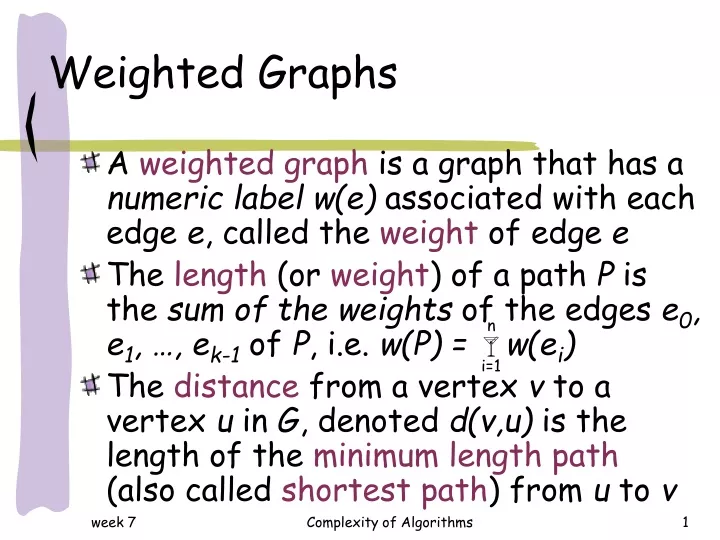
n. . i=1. Weighted Graphs. A weighted graph is a graph that has a numeric label w(e) associated with each edge e , called the weight of edge e The length (or weight ) of a path P is the sum of the weights of the edges e 0 , e 1 , …, e k-1 of P , i.e. w(P) = w(e i )

E N D
n i=1 Weighted Graphs • A weighted graph is a graph that has a numeric label w(e) associated with each edge e, called the weight of edge e • The length (or weight) of a path P is the sum of the weights of the edges e0, e1, …, ek-1 of P, i.e. w(P) = w(ei) • The distance from a vertex v to a vertex u in G, denoted d(v,u) is the length of the minimum length path (also called shortest path) from u to v Complexity of Algorithms
Single-Source Shortest Paths • Suppose we are given a weighted graph, and we are asked to find a shortest path from some vertex v to each other vertex in G, viewing the weights on the edges as distances • This problem is called a single-source shortest paths problem, in short SSSP Complexity of Algorithms
Greedy Approach to SSSP • There is an interesting approach for solving the SSSP based on the greedy method design pattern • The main idea in applying the greedy method pattern to the SSSP is to perform a ‘’weighted’’ BFS • An algorithm using this design pattern is known as Dijkstra’s algorithm Complexity of Algorithms
Dijkstra’s Algorithm • We assume that all edges in the graph have non-negative weights • Let v be a source vertex and let D[u] represent the temporary distance in G from v to u, where initially D[v] = 0 and D[u] = + , for v u • Initially all entries in array D are temporary, but after each stage of the algorithm one entry in D becomes fixed Complexity of Algorithms
Edge Relaxation • Assume that C is a set of vertices for which entries in array D are already fixed (i.e., the shortest distances between v and vertices in C has been found), and that entry D[u] was fixed in the last round • At any vertex z, s.t., the value of D[z] is not fixed yet, perform the edge relaxation • If D[u] + w((u,z)) < D[z] then • D[z] D[u] + w((u,z)) Complexity of Algorithms
Fixing next D entry • When the edge relaxation is completed • fix one entry in G (among vertices still outside of C) with the smallest weight currently available • then proceed to the next stage of edge relaxation based on extended set of vertices C (with fixed entries) Complexity of Algorithms
Dijkstra’s Algorithm D [ a b c d e f ] C f 1 x x x 0 x x a 4 x x 4 02 x {d} 1 4 b x 6 302 6 {d,e} e 4 4 7 4302 6 {c,d,e} 1 1 7 43025{b,c,d,e} 2 c 643025{b,c,d,e,f} 4 d 643025{a,b,c,d,e,f} Complexity of Algorithms
Dijkstra’s Alg. (pseudo-code) Complexity of Algorithms
Dijkstra’s Alg. (complexity) • Let G=(V,E), where ¦V¦=n & ¦E¦=m • Entries of array D for vertices outside of C (not fixed yet) are stored in a PQ, i.e., each access to such entry costs O(log n) • Penetration of a new edge (in edge relaxation stage) requires a single access to the PQ Complexity of Algorithms
Dijkstra’s Alg. (complexity) • Theorem: • Given a weighted graph with n vertices and m edges, each with a non-negative weight. • Dijkstra’s algorithm (that finds all shortest paths from a distinguished vertex v) can be implemented in time O(m log n) Complexity of Algorithms
The Bellman-Ford Algorithm • There is another algorithm, which is due to Bellman and Ford, that can find shortest paths in graphs that have negative-weight edges • However, we must assume in this case that the graph is directed (otherwise we could traverse along a negative-weight edge back and forth for as long as we needed ending up with a path as light as we wanted) Complexity of Algorithms
The Bellman-Ford Algorithm • The Bellman-Ford algorithm shares the notion of edge relaxation from Dijkstra’s algorithm, however • It does not use it in conjunction with the greedy method, but rather • Performs a relaxation of every edge in a digraph exactly (n-1) times Complexity of Algorithms
The BF Algorithm (pseudo-code) Complexity of Algorithms
The BF algorithm (example) Complexity of Algorithms
The BF algorithm (example) Complexity of Algorithms
The BF algorithm (example) Complexity of Algorithms
The BF algorithm (analysis) • The Bellman-Ford algorithm is divided into n-1 stages, s.t., after stage i, for i= 1, …, n-1, the shortest paths made of at most i edges are computed • During each stage i every edge takes part in edge relaxation at most once • The longest shortest (lightest) path (excluding a negative cycle) is of length n-1 Complexity of Algorithms
The BF algorithm (analysis) • Theorem: Given a directed graph G with n vertices and m edges, and a vertex v of G. • The Bellman-Ford algorithm computes the distance from v to all other vertices of G, or • Determine that G contains a negative-weight cycle, • In O(nm) time Complexity of Algorithms
Minimum Spanning Tree (MST) • Given undirected graph G • We are interested in finding a tree T • that contains all the vertices in G, and • minimises the sum of the weights of the edges of T, i.e., w(T) = w(e) • Computing a spanning tree T with smallest total weight is the problem of constructing a minimum spanning tree or MST e T Complexity of Algorithms
Prim’s MST Algorithm D [ a b c d e f ] C (edges) x x 4 02 x f 4 a x 4 100 6 {(d,e)} 6 1 3 2000 4 {(d,e), (e,c)} 4 b e 4 3 3 00001{(d,e), (e,c), (c,b)} 2 300000{(d,e), (e,c), (c,b), (b,f)} 1 2 c 000000{(d,e), (e,c), (c,b), (b,f), (c,a)} 4 d Total = 2 + 1 + 2 + 1 + 3 = 9 Complexity of Algorithms
Prim’s Algorithm (pseudo-code) Complexity of Algorithms
Prim’s MST Algorithm • Theorem: Given a simple connected weighted graph G with n vertices and m edges • the Prim’s algorithm finds a minimum spanning tree for G • In O(m log n) time Complexity of Algorithms
Kruskal’s MST Algorithm f 4 4 a 6 6 1 1 4 4 b e 4 4 3 3 Invariant: Always pick the lightest edge that doesn’t create a cycle 2 2 1 1 2 2 c 4 4 Total weight = 1 + 1 + 2 + 2 + 3 = 9 d Complexity of Algorithms
Kruskal’s Alg. (pseudo-code) Complexity of Algorithms
Kruskal’s MST Algorithm • Theorem: Given a simple connected weighted graph G with n vertices and m edges • the Kruskal’s algorithm finds a minimum spanning tree for G • In O((n+m) log n) time Complexity of Algorithms
Barůvka’s MST Algorithm • Barůvka’s algorithm is a combination of Kruskal’s and Prim’s MST algorithms, i.e., • as in Kruskal’s algorithm it builds the MST by growing a number of clusters simultaneously, and • as in Prim’s algorithm it extends (each) cluster adding one outgoing edge that possibly joins two clusters Complexity of Algorithms
Barůvka’s Alg. (pseudo-code) Complexity of Algorithms
Barůvka’s Algorithm (example) Complexity of Algorithms
Barůvka’s Algorithm (complexity) • Theorem: Given a simple connected weighted graph G with n vertices and m edges • the Barůvka’s algorithm finds a minimum spanning tree for G • In O(m log n) time Complexity of Algorithms