Download
1 / 32
320 likes | 347 Vues
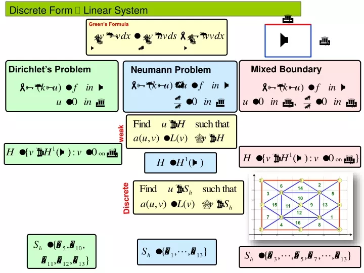
Discrete Form Linear System. Green’s Formula. Mixed Boundary. Dirichlet’s Problem. Neumann Problem. weak. Discrete. Discrete Form Linear System. Its weak form. Dirichlet’s Problem. (x^2-x)(1-4y-2x)+(y^2-y)(1-4x-2y). Remark:. The approximate Solution. Remark:.

E N D
Discrete Form Linear System Green’s Formula Mixed Boundary Dirichlet’s Problem Neumann Problem weak Discrete
Discrete Form Linear System Its weak form Dirichlet’s Problem (x^2-x)(1-4y-2x)+(y^2-y)(1-4x-2y) Remark:
The approximate Solution Remark: This matrix is sparse (many zeros) few non-zero entries
Sparsity In Matrix form Remark: This matrix is sparse (many zeros) few non-zero entries another example
Sparsity Sparsity of the matrix # of nonzero =1153 312 triangles and 177nodes Use spy(A) to see sparsity
Remark: Assembly of the Stiffness Matrix These few nonzero entries are computed by looping over all triangles In Matrix form Remark: nonzero entry is a sum of integrals of local basis functions over a triangle
Assembly of the Stiffness Matrix Step1 primary stiffnes matrix Loop over all triangles 1 -16. in each triangle, we calculate 3x3 matrix which involves calculating 9 integrals of all possible combination of local basis functions. Step2 impose boundary condition After we assemble the primary stiffness matrix in step1, we enforce the boundary condition by forcing the corresponding coefficient to be zero.
Step1 primary stiffnes matrix For k = 1 : 16 Step1a: find all gradients Step1b: Find 9 integrals Step1c: Add these contributions to the primary stiffness matrix End the loop
Find the gradients with cyclic permutation of the index i,j k over 1,2,3 Remark:
Find the gradients Remark: function [area,b,c] = Gradients(x,y) area=polyarea(x,y); b=[y(2)-y(3); y(3)-y(1); y(1)-y(2)]/2/area; c=[x(3)-x(2); x(1)-x(3); x(2)-x(1)]/2/area;
Step1 primary stiffnes matrix Loop over all triangles 1 -16 for example K9 10 5 13
Numerical Integration 1D Mid-point Quadrature 2D 2D
Quadrature in a Triangle K Mid-point Quadrature 1 Node quadrature 2
Step1 primary stiffnes matrix Use Gradients(x,y) We want to compute: local basis functions 10 5 13 Element stiffnes matrix Element stiffnes matrix
10 5 13 Local to global
Triangle K10 1 2 3 1 7/6 -7/12 -7/2 2 -7/12 7/12 0 3 -7/12 0 7/12 Local to global 5 10 11 5 7/6 -7/12 -7/2 10 -7/12 7/12 0 11 -7/12 0 7/12
K1 = 0.4167 0 -0.4167 0 0.4167 -0.4167 -0.4167 -0.4167 0.8333 K2 = 0.1667 0 -0.1667 0 0.1667 -0.1667 -0.1667 -0.1667 0.3333 K3 = 0.5833 0 -0.5833 0 0.5833 -0.5833 -0.5833 -0.5833 1.1667 K14 = 0.3333 0 -0.3333 0 0.3333 -0.3333 -0.3333 -0.3333 0.6667 K15 = 0.6667 0 -0.6667 0 0.6667 -0.6667 -0.6667 -0.6667 1.3333 K16 = 0.6667 0 -0.6667 0 0.6667 -0.6667 -0.6667 -0.6667 1.3333
12 0 0 0 0 0 0 0 0 0 36 0 0 0 0 0 0 0 0 0 60 0 0 0 0 0 0 0 0 0 36 0 0 0 0 0 0 0 0 0 144 0 0 0 0 0 0 0 0 0 45 0 0 0 0 0 0 0 0 0 99 0 0 0 0 0 0 0 0 0 99 0 0 0 0 0 0 0 0 0 45 -12 0 0 0 -30 -18 0 0 -18 0 -36 0 0 -36 -27 -45 0 0 0 0 -60 0 -42 0 -54 -54 0 0 0 0 -36 -36 0 0 -45 -27 -12 0 0 0 0 -36 0 0 0 0 -60 0 0 0 0 -36 -30 -36 -42 -36 -18 -27 0 0 0 -45 -54 0 0 0 -54 -45 -18 0 0 -27 78 0 0 0 0 144 0 0 0 0 210 0 0 0 0 144
Step1 primary stiffnes matrix function K = StiffMat2D(p,t) k = inline('x+y','x','y'); np = size(p,2); nt = size(t,2); K = sparse(np,np); for m = 1:nt loc2glb = t(1:3,m); % local-to-global map x = p(1,loc2glb); % node x-coordinates y = p(2,loc2glb); % node y-coordinates [area,b,c] = Gradients(x,y); xc = mean(x); yc = mean(y); kc = k(xc,yc); Ke = (b*b'+c*c')*area*kc; % element stiff mat K(loc2glb,loc2glb) = K(loc2glb,loc2glb)+ Ke; % add element stiff to K end
Assemble the Load vector L In Matrix form
Assembly of the Load Vector Step1 primary Load vector Loop over all triangles 1 -16. in each triangle, we calculate 3x1 matrix which involves calculating 3 integrals Step2 impose boundary condition After we assemble the primary load vector and stiffness matrix in step1, we enforce the boundary condition by forcing the corresponding coefficient to be zero.
2 Step1 primary Load vector Loop over all triangles 1 -16. in each triangle, we calculate 3x1 matrix which involves calculating 3 integrals The load vector L is assembled using the same technique as the primary stiffness matrix A, that is, by summing element load vectors LKover the mesh. On each element K we get a local 3×1 element load vector BKwith entries LKi = ∫Kf φi dx; i = 1;2;3 Using node quadrature, we compute these integrals we end up with LKi≈ 1/3f (Ni)|K|; i = 1;2;3
Step1 primary Load vector Loop over all triangles 1 -16. in each triangle, we calculate 3x1 matrix which involves calculating 3 integrals
Step1 primary Load vector Loop over all triangles 1 -16. in each triangle, we calculate 3x1 matrix which involves calculating 3 integrals
Step1 primary Load vector Loop over all triangles 1 -16. in each triangle, we calculate 3x1 matrix which involves calculating 3 integrals 0 0 1/24 0 1/48 0 1/32 1/32 0 1/128 3/128 9/128 3/128 L1 = 0 0 1/256 . . . L16 = 1/256 3/256 1/96 We summarize the computation of the load vector with the following Matlab code. function L = LoadVec2D(p,t) f = inline('(x.^2-x).*(1-4*y-2*x)+(y.^2-y).*(1-4*x-2*y)','x','y'); np = size(p,2); nt = size(t,2); L = zeros(np,1); for K = 1:nt loc2glb = t(1:3,K); x = p(1,loc2glb); y = p(2,loc2glb); area = polyarea(x,y); bK = [f(x(1),y(1));f(x(2),y(2));f(x(3),y(3))]/3*area; % element load vector L(loc2glb) = L(loc2glb)+ bK; % add element loads to b end
c1 c2 c3 c4 c5 c6 c7 c8 c9 c10 c11 c12 c13 c1 c2 c3 c4 c5 c6 c7 c8 c9 c10 c11 c12 c13 0 0 0 0 1/12 0 1/16 1/16 0 3/128 3/32 21/128 3/32 0 0 0 0 1/12 0 1/16 1/16 0 3/128 3/32 21/128 3/32 12 0 0 0 0 0 0 0 0 0 36 0 0 0 0 0 0 0 0 0 60 0 0 0 0 0 0 0 0 0 36 0 0 0 0 0 0 0 0 0 144 0 0 0 0 0 0 0 0 0 45 0 0 0 0 0 0 0 0 0 99 0 0 0 0 0 0 0 0 0 99 0 0 0 0 0 0 0 0 0 45 -12 0 0 0 -30 -18 0 0 -18 0 -36 0 0 -36 -27 -45 0 0 0 0 -60 0 -42 0 -54 -54 0 0 0 0 -36 -36 0 0 -45 -27 12 0 0 0 0 0 0 0 0 0 36 0 0 0 0 0 0 0 0 0 60 0 0 0 0 0 0 0 0 0 36 0 0 0 0 0 0 0 0 0 144 0 0 0 0 0 0 0 0 0 45 0 0 0 0 0 0 0 0 0 99 0 0 0 0 0 0 0 0 0 99 0 0 0 0 0 0 0 0 0 45 -12 0 0 0 -30 -18 0 0 -18 0 -36 0 0 -36 -27 -45 0 0 0 0 -60 0 -42 0 -54 -54 0 0 0 0 -36 -36 0 0 -45 -27 -12 0 0 0 0 -36 0 0 0 0 -60 0 0 0 0 -36 -30 -36 -42 -36 -18 -27 0 0 0 -45 -54 0 0 0 -54 -45 -18 0 0 -27 78 0 0 0 0 144 0 0 0 0 210 0 0 0 0 144 -12 0 0 0 0 -36 0 0 0 0 -60 0 0 0 0 -36 -30 -36 -42 -36 -18 -27 0 0 0 -45 -54 0 0 0 -54 -45 -18 0 0 -27 78 0 0 0 0 144 0 0 0 0 210 0 0 0 0 144 = = Impose Boundary Conditions
Step2 impose boundary condition c1 c2 c3 c4 c5 c6 c7 c8 c9 c10 c11 c12 c13 0 0 0 0 1/12 0 1/16 1/16 0 3/128 3/32 21/128 3/32 This can be done in Matlab: function [A,b] = impose_boundary(A,b,p,t,e); np = size(p,2); % total number of nodes bound = e(1,:); % boundary nodes for i=1:length(e) ib = bound(i); A(ib,:)=sparse(1,np); A(:,ib)=sparse(np,1); A(ib,ib)=1; b(ib)=0; end 12 0 0 0 0 0 0 0 0 0 36 0 0 0 0 0 0 0 0 0 60 0 0 0 0 0 0 0 0 0 36 0 0 0 0 0 0 0 0 0 144 0 0 0 0 0 0 0 0 0 45 0 0 0 0 0 0 0 0 0 99 0 0 0 0 0 0 0 0 0 99 0 0 0 0 0 0 0 0 0 45 -12 0 0 0 -30 -18 0 0 -18 0 -36 0 0 -36 -27 -45 0 0 0 0 -60 0 -42 0 -54 -54 0 0 0 0 -36 -36 0 0 -45 -27 -12 0 0 0 0 -36 0 0 0 0 -60 0 0 0 0 -36 -30 -36 -42 -36 -18 -27 0 0 0 -45 -54 0 0 0 -54 -45 -18 0 0 -27 78 0 0 0 0 144 0 0 0 0 210 0 0 0 0 144 =
Main file exact U %Main.m files %load sample_mesh np = size(p,2); K = StiffMat2D(p,t); L = LoadVec2D(p,t); Lo=L; A = K; [A,L] = impose_boundary(A,L,p,t,e); U = zeros(np,1); % allocate solution vector U = A\L; % solve the linear system x=0:0.01:1; y=0:0.01:1; u=tri2grid(p,t,U,x,y); mesh(x,y,u) % plot surface uexact = inline('(x-x.^2).*(y-y.^2)','x','y'); ue = uexact(p(1,:),p(2,:))'; [U,ue] norm(U-ue) figure; ezsurf('(x.^2-x).*(y.^2-y)',[0,1],[0,1]) 0 0 0 0 0 0 0 0 0.0584 0.0625 0 0 0 0 0 0 0 0 0.0333 0.0352 0.0380 0.0352 0.0398 0.0352 0.0380 0.0352
Step2 impose boundary condition x=0:0.01:1; y=0:0.01:1; u=tri2grid(p,t,c,x,y); mesh(x,y,u)
1 (due 17Feb) Suppose the model equation of a physical problem is given by Use the following mesh to : 8 7 6 2 1 3 4 5 3) Find the element load vector for the triangle K5. Use two different formula for the quadrature (show all your work) 1) Find the matrices p, e, t. 2) Find the element stiffness matrix for the triangle K6 and K8 (show all your work) 4) Assemble the primary stiffness matrix A and the primary load vector b.