Download
1 / 19
190 likes | 805 Vues
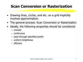
Scan Conversion or Rasterization. Drawing lines, circles, and etc. on a grid implicitly involves approximation. The general process: Scan Conversion or Rasterization Ideally, the following properties should be considered smooth continuous pass through specified points uniform brightness

E N D
Scan Conversion or Rasterization • Drawing lines, circles, and etc. on a grid implicitly involves approximation. • The general process: Scan Conversion or Rasterization • Ideally, the following properties should be considered • smooth • continuous • pass through specified points • uniform brightness • efficient 168 471 Computer Graphics, KKU. Lecture 6
Line Drawing and Scan Conversion • There are three possible choices which are potentially useful. • Explicit: y = f(x) • y = m (x - x0) + y0 where m = dy/dx • Parametric: x = f(t), y = f(t) • x = x0 + t(x1 - x0), t in [0,1] • y = y0 + t(y1 - y0) • Implicit: f(x, y) = 0 • F(x,y) = (x-x0)dy - (y-y0)dx • if F(x,y) = 0 then (x,y) is on line • F(x,y) > 0 then (x,y) is below line • F(x,y) < 0 then (x,y) is above line 168 471 Computer Graphics, KKU. Lecture 6
Line Drawing - Algorithm 1 A Straightforward Implementation DrawLine(int x1,int y1, int x2,int y2, int color) { float y; int x; for (x=x1; x<=x2; x++) { y = y1 + (x-x1)*(y2-y1)/(x2-x1) WritePixel(x, Round(y), color ); } } 168 471 Computer Graphics, KKU. Lecture 6
Line Drawing - Algorithm 2 A Better Implementation DrawLine(int x1,int y1,int x2,int y2, int color) { float m,y; int dx,dy,x; dx = x2 - x1; dy = y2 - y1; m = dy/dx; y = y1 + 0.5; for (x=x1; x<=x2; x++) { WritePixel(x, Floor(y), color ); y = y + m; } } 168 471 Computer Graphics, KKU. Lecture 6
Line Drawing Algorithm Comparison • Advantages over Algorithm 1 • eliminates multiplication • improves speed • Disadvantages • round-off error builds up • get pixel drift • rounding and floating point arithmetic still time consuming • works well only for |m| < 1 • need to loop in y for |m| > 1 • need to handle special cases 168 471 Computer Graphics, KKU. Lecture 6
Line Drawing - Midpoint Algorithm • The Midpoint or Bresenham’s Algorithm • The midpoint algorithm is even better than the above algorithm in that it uses only integer calculations. It treats line drawing as a sequence of decisions. For each pixel that is drawn the next pixel will be either N or NE, as shown below. 168 471 Computer Graphics, KKU. Lecture 6
Midpoint Algorithm • The midpoint algorithm makes use of the implicit definition of the line, F(x,y) =0. The N/NE decisions are made as follows. • d = F(xp + 1, yp + 0.5) • if d < 0 line below midpoint choose E • if d > 0 line above midpoint choose NE • if E is chosen • dnew = F(xp + 2, yp + 0.5) • dnew- dold = F(xp + 2, yp + 0.5) - F(xp + 1, yp + 0.5) • Delta = d new -d old = dy 168 471 Computer Graphics, KKU. Lecture 6
Midpoint Algorithm • If NE is chosen • dnew = F(xp+2, yp+1.5) • Delta = dy-dx • Initialization • dstart = F(x0+1, y0+0.5) = (x0+1-x0)dy - (y0+0.5-y0)dx = dy-dx/2 • Integer only algorithm • F’(x,y) = 2 F(x,y) ; d’ = 2d • d’start = 2dy - dx • Delta’ = 2Delta 168 471 Computer Graphics, KKU. Lecture 6
Midpoint Algorithm for x1 < x2 and slope <= 1 DrawLine(int x1, int y1, int x2, int y2, int color) { int dx, dy, d, incE, incNE, x, y; dx = x2 - x1; dy = y2 - y1; d = 2*dy - dx; incE = 2*dy; incNE = 2*(dy - dx); y = y1; for (x=x1; x<=x2; x++) { WritePixel(x, y, color); if (d>0) { d = d + incNE; y = y + 1; } else { d = d + incE; } } } 168 471 Computer Graphics, KKU. Lecture 6
General Bressenham’s Algorithm • To generalize lines with arbitrary slopes • consider symmetry between various octants and quadrants • for m > 1, interchange roles of x and y, that is step in y direction, and decide whether the x value is above or below the line. • If m > 1, and right endpoint is the first point, both x and y decrease. To ensure uniqueness, independent of direction, always choose upper (or lower) point if the line go through the mid-point. • Handle special cases without invoking the algorithm: horizontal, vertical and diagonal lines 168 471 Computer Graphics, KKU. Lecture 6
Scan Converting Circles • Explicit: y = f(x) Usually, we draw a quarter circle by incrementing x from 0 to R in unit steps and solving for +y for each step. • Parametric: - by stepping the angle from 0 to 90 - avoids large gaps but still insufficient. • Implicit: f(x) = x2+y2-R2 If f(x,y) = 0 then it is on the circle. f(x,y) > 0 then it is outside the circle. f(x,y) < 0 then it is inside the circle. 168 471 Computer Graphics, KKU. Lecture 6
Eight-way Symmetry 168 471 Computer Graphics, KKU. Lecture 6
dold = F(xp+1, yp+0.5) If dold < 0, E is chosen dnew = F(xp+2, yp-0.5) = dold+(2xp+3) DeltaE = 2xp+3 If dold >= 0, SE is chosen dnew = F(xp+2, yp-1.5) = dold+(2xp-2yp+5) DeltaSE = 2xp-2yp+5 Initialization dinit = 5/4 – R = 1 - R Midpoint Circle Algorithm 168 471 Computer Graphics, KKU. Lecture 6
Midpoint Circle Algorithm (cont.) 168 471 Computer Graphics, KKU. Lecture 6
Scan Converting Ellipses • 2a is the length of the major axis along the x axis. • 2b is the length of the minor axis along the y axis. • The midpoint can also be applied to ellipses. • For simplicity, we draw only the arc of the ellipse that lies in the first quadrant, the other three quadrants can be drawn by symmetry 168 471 Computer Graphics, KKU. Lecture 6
Firstly we divide the quadrant into two regions • Boundary between the two regions is • the point at which the curve has a slope of -1 • the point at which the gradient vector has the i and j components of equal magnitude j > i in region 1 j < i in region 2 Scan Converting Ellipses: Algorithm 168 471 Computer Graphics, KKU. Lecture 6
Ellipses: Algorithm (cont.) • At the next midpoint, if a2(yp-0.5)<=b2(xp+1), we switch region 1=>2 • In region 1, choices are E and SE • Initial condition: dinit = b2+a2(-b+0.25) • For a move to E, dnew = dold+DeltaE with DeltaE = b2(2xp+3) • For a move to SE, dnew = dold+DeltaSE with DeltaSE = b2(2xp+3)+a2(-2yp+2) • In region 2, choices are S and SE • Initial condition: dinit = b2(xp+0.5)2+a2((y-1)2-b2) • For a move to S, dnew = dold+Deltas with Deltas = a2(-2yp+3) • For a move to SE, dnew = dold+DeltaSE with DeltaSE = b2(2xp+2)+a2(-2yp+3) • Stop in region 2 when the y value is zero. 168 471 Computer Graphics, KKU. Lecture 6
Midpoint Ellipse Algorithm 168 471 Computer Graphics, KKU. Lecture 6
Midpoint Ellipse Algorithm (cont.) 168 471 Computer Graphics, KKU. Lecture 6