Download
1 / 21
220 likes | 248 Vues
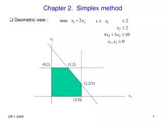
Chapter 2. Simplex method. Geometric view :. x 2. (0,2). (1,2). (2,2/3). x 1. (2,0). Let a R n , b R. Geometric intuition for the solution sets of { x : a’x = 0 } { x : a’x 0 } { x : a’x 0 } { x : a’x = b } { x : a’x b } { x : a’x b }.

E N D
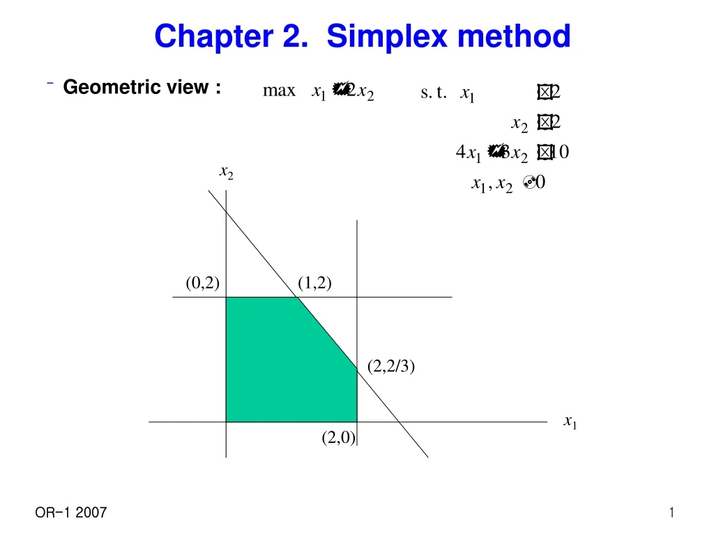
Chapter 2. Simplex method • Geometric view : x2 (0,2) (1,2) (2,2/3) x1 (2,0)
Let a Rn, b R. Geometric intuition for the solution sets of { x : a’x = 0 } { x : a’x 0 } { x : a’x 0 } { x : a’x = b } { x : a’x b } { x : a’x b }
{ x : a’x 0 } { x : a’x = 0 } { x : a’x 0 } • Geometry in 2-D a 0
Let z be a (any) point satisfying a’x = b. Then { x : a’x = b } = { x : a’x = a’z } = { x : a’(x – z) = 0 } Hence x – z = y, where y is any solution to a’y = 0, or x = y + z. So x can be obtained by adding z to every point y satisfying Ay = 0. Similarly, for { x : a’x b }, { x : a’x b }. { x : a’x b } a z 0 { x : a’x = b } { x : a’x b } { x : a’x = 0 }
(2,2/3) • Points satisfying (halfspace) x2 (4,3) x1
Def: The set of points which can be described in the form is called a polyhedron. ( Intersection of finite number of halfspaces) Hence, linear programming is the problem of optimizing (maximize, minimize) a linear function over a polyhedron. • Thm) Polyhedron is a convex set. Pf) HW
Solving LP graphically x2 (0,2) (1,2) (2,2/3) x1 (2,0)
Properties of optimal solution • Thm) If LP has a unique optimal solution, the optimal solution is an extreme point. Pf) Suppose x* is unique optimal solution and it is not extreme point of the feasible set. Then there exist feasible points y, z x* such that x* = y +(1- )z for some 0 < < 1. Then c’x* = c’y + (1- )c’z. If c’x* c’y, then either c’y > c’x* or c’z > c’x*, hence contradiction to x* being optimal solution. If c’x* = c’y, y is also optimal solution. Contradiction to x* being unique optimal. • Thm) Suppose polyhedron P has at least one extreme point. If LP over Phas an optimal solution, it has an extreme point optimal solution. Pf) not given here.
Multiple optimal solutions x2 (0,2) (1,2) (2,2/3) x1 (2,0)
Obtaining extreme point algebraically x2 (0,2) (1,2) (2,2/3) x1 (2,0)
Suppose polyhedron is given (A: mxn). Extreme point of the polyhedron can be obtained by setting n of the inequalities as equations (coefficient vectors must be linearly independent) and obtaining the solution satisfying the equations. If the obtained point satisfies other inequalities, it is in P and it is an extreme point of the polyhedron • Enumeration : ( the number of ways to choose n inequalities (which hold at equalities) out of (m+n) inequalities.) • Algorithm strategy : from an extreme point, move to the neighboring extreme point which gives a better (precisely speaking, not worse) solution
주의 : full dimension이 아닌 polyhedron 도 존재 가능(extreme point?) x3 1 x1 1 This polyhedron is 2-dimensional. 1 x2
Geometric Idea of the Simplex Method • Any LP problem must be converted to a problem having only equations except the nonnegativity constraints if simplex method can be applied (방법은 뒤에) • Consider the LP problem max c’x, Ax = b, -x 0 A: m n, full row rank(n m) P = { x : Ax=b, -x 0 } To define an extreme point of P, we need n equations. Since we already have mequations Ax=b, (n - m) equations must come from -x 0, which means (n - m) variables are set at 0. Let A=[B:N], where N is the submatrix corresponding to the variables set at 0. Then we solve the system Bx = b for the remaining m variables. (Note that the coefficient matrix B must be nonsingluar so that the system of equations has a unique solution.)
Ex: extreme point ( 1, 0, 0 ) can be obtained from x1 + x2 + x3 = 1, x2 = 0, x3 = 0. Since ( 1, 0, 0 ) satisfies –x1 0, it is an extreme point. x3 1 x1 1 This polyhedron is 2-dimensional. 1 x2
(continued) Let A = [B : N] , B: m m, nonsingular, N: m (n - m), where N is the submatrix of A having columns associated with variables set at 0. Then the extreme point can be found by solving Ax = b, xN = 0. [B : N] (xB: xN)’ = b BxB + NxN = b, -xN = 0. (or BxB = b - NxN , -xN = 0. ) solution is xB = B-1b, xN = 0 This is the basic solution we mentioned earlier. By the choice of the variables we set at 0, we obtain different basic solutions (different extreme points). If the obtained solution satisfies xB = B-1b 0, we have a basic and feasible solution (satisfies nonnegativity of variables) • Simplex method searches only basic solutions (and feasible), which is tantamount to searching the extreme points of the underlying polyhedron until it finds an optimal solution.
Simplex method (algebraic interpretation) Add slack variables(여유변수) to each constraint to convert them to equations. (1) (2)
Hence we have a 1-1 mapping which maps each feasible point in (1) to a feasible point in (2) uniquely (and conversely) and the objective values are the same for the points. So solve (2) instead of (1). (Surplus variable (잉여변수) : a’x b a’x – xs =b, xs 0)
참고: 제약식에 등식이 있을 경우, 이를 두개의 부등식으로 표현하여 여유변수나 잉여변수를 더하여 등식으로 표현하면 되나 이런 경우 제약식의 숫자가 늘어나서 문제를 푸는데 걸리는 시간이 늘어날 수 있음. 등식을 두개의 부등식으로 표현하지 않고 바로 처리할 수 있는 방법도 있으며 이에 대해서는 나중에 설명. (Chap 8. General LP Problems)
여유변수의 도입에 따른 해공간의 변화 x2 x3 1 1 x1 1 1 x1 1 x2
Next let Then find solution to the following system which maximizes z (tableau form) In the text, dictionary form used, i.e. each dependent variable (including z) is expressed as linear combinations of indep. var.) (Note that, unlike the text, we place the objective function in the first row. Such presentation style is used more widely and we follow that convention)
From previous lectures, we know that if the polyhedron P has at least one extreme point and the LP over P has a finite optimal solution, the LP has an extreme point optimal solution. Also an extreme point of P for our problem is a basic feasible solution algebraically. We obtain a basic solution by setting x1 = x2 = x3 = 0 and finding the values of x4, x5, and x6 , which can be read directly from the dictionary. (also z values can be read.) If all values of x4, x5, and x6 are nonnegative, we obtain a basic feasible solution. • The equation for z may be regarded as part of the systems of equations, or we may think of it as a separate equation used to evaluate the objective value for the given solution.