Download
1 / 11
110 likes | 237 Vues
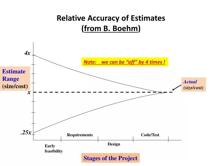
Relative Accuracy of Estimates ( from B. Boehm ). 4x. Note: we can be “off” by 4 times !. Estimate Range (size/cost). Actual (size/cost). x. .25x. Requirements. Code/Test. Design. Early feasibility. Stages of the Project. More “Modern” version of FP.

E N D
Relative Accuracy of Estimates(from B. Boehm) 4x Note: we can be “off” by 4 times ! Estimate Range (size/cost) Actual (size/cost) x .25x Requirements Code/Test Design Early feasibility Stages of the Project
More “Modern” version of FP Composed of 3 major steps: • Identify and Classifying: • Data • Transactions • Evaluation of Complexity Levels of Data and Transactions • Compute the Functional Point
1. Identifying & Classifying 5 “Basic Entities” • Data: • Internally generated and stored (logical files and tables) • Data maintained externally and requires an external interface to access (external interfaces) • Transactions: • Information or data entry into a system for transaction processing (inputs) • Information or data “leaving” the system such as reports or feeds to another application (outputs) • Information or data retrieved and displayed on the screen in response to query (query)
2. Evaluating Complexity • Using a complexity table, each of the 5 basic entities is evaluated as : • Low (simple) • Average • High (complex) • 3 attributes are used for the above complexity table decisions • # ofRecord Element Types (RET): e.g. employee data type, student record type • # of unique attributes (fields) or Data Element Types (DET) for each record : e.g. name, address, employee number, and hiring date would make 4 DETs for employee data stype • # ofFile Type Referenced (FTR): e.g an external payroll record file that needs to be accessed
5 Basic Entity Types uses the RET, DET, and FTRfor Complexity Evaluation For -- Internal Logical Files and External Interfacesdata entities: # of RET1-19 DET20-50 DET50+ DET 1 Low Low Ave 2 -5 Low Avg High 6+ Avg High High For -- Input, Output and Query transactions: # of FTR1-4 DET5 -15 DET16+ DET 0 - 1 Low Low Ave 2 Low Avg High 3+ Avg High High
Example • Consider a requirement: “has the feature to add a new employee to the “system.” • Assume employee information involves 3 external files that each has a different Record Element Types (RET) • Employee Basic Information has employee data records • Each employee record has 55 fields (1 RET and 55 DET) - AVERAGE • Employee Benefits records • Each benefit record has 10 fields (1 RET and 10 DET) - LOW • Employee Tax records • Each tax record has 5 fields ( 1 RET and 5 DET) - LOW • Adding a new employee involves 1 input transaction which involves 3 file types referenced (FTR) and a total of 70 fields (DET). So for the 1 input transaction the complexity is HIGH
Function Point (FP) Computation • Composed of 5 “Basic Entities” • input items (external input items from user or another application) • output items (external outputs such as reports, messages, screens – not each data item) • Queries (a query that results in a response of one or more data) • master and logical files (internal file or data structure or data table) • external interfaces (data or sets of data sent to external devices, applications, etc.) • And a “complexity level index” matrix : Simple(low) Complex (high) Average 3 4 6 Input 5 7 Output 4 3 Query 4 6 Logical files 7 10 15 Ext. Interface & file 7 5 10
Function Point Computation (cont.) • Initial Function Point : Σ [Basic Entity x Complexity Level Index] all basic entities Continuing the Example of adding new employee: - 1 external interface (average) = 7 - 1 external interface (low) = 5 - 1 external interface (low) = 5 - 1 input (high) = 6 Initial Function Point = 7 + 5 + 5 + 6 = 23 Note that ---- this just got us to Initial Function Point
Function Point Computation (cont.) • Initial Function Point : ∑ (Basic Entity x Complexity Level Index) is modified by 14 DI’s • There are 14 more “Degree of Influences” ( 0 to 5 scale) : • data communications • distributed data processing • performance criteria • heavy hardware utilization • high transaction rate • online data entry • end user efficiency • on-line update • complex computation • reusability • ease of installation • ease of operation • portability • maintainability These form the 14 DIs
Function Point Computation (cont.) • Define Technical Complexity Factor (TCF): • TCF = .65 + [(.01) x (14 DIs )] • where DI = ∑ ( influence factor value) • So note that .65 ≤ TCF ≤ 1.35 Function Point (FP) = Initial FP x TCF Finishing the earlier Example: for the example, assume TCF came out to be 1.15, then Function Point = 23 x 1.15 = 26.45
Function Point • Provides you another way to estimate the “size” of the project based on estimating 5 basic entities : • Inputs • Outputs • Logical Files • External Interfaces • Queries • (note : the text book algorithm is earlier, simplified version) (important) • ** Then --- still need to have an estimate on productivity e.g. function point/person-month • ***Divide the estimated total project function points (size) by the productivity to get an estimate of “effort” in person-month or person-days needed. - - - - - - - - - - - - - - - - - - - - - - - -