Download
1 / 18
180 likes | 292 Vues
EV vs. CV. EV - how much more money a consumer would pay before a price increase to avert the price increase CV - the amount of additional money an agent would need to reach its initial utility after a change in prices, or a change in product quality, or the introduction of new products.

E N D
EV vs. CV • EV - how much more money a consumer would pay before a price increase to avert the price increase • CV - the amount of additional money an agent would need to reach its initial utility after a change in prices, or a change in product quality, or the introduction of new products
Assumptions • Natural monopoly • Cost minimization requires one firm in the market • Strong natural monopoly • MC pricing crease deficit • MC with subsidies is not an option • Barriers to entry • Product demands are unrelated (we relax this assumption later in more complex models)
Regulation • Objective is to maximize social welfare subject to the firm breaking even • Per unit charge (constant price) • Prices across markets can vary • First best pricing is not an option • Second best (Ramsey Prices) based on maximizing welfare subject to an acceptable level of profit
Ramsey Prices • Where • the percentage deviation of price from marginal cost in the ith market should be inversely proportional to the absolute value of demand elasticity in the ith market
They were developed in a partial-equilibrium framework in which only one multiproduct firm as considered. There were no competitors in any markets, and all cross-elasticitiesof demand were zero. • Consider a more relaxed assumption. • The firm is still classified as a strong natural monopoly, but faces competition in some of its output markets. • Some of its outputs are imperfect substitutes or imperfect complements to outputs produced in the private sector. • Cross-elasticities of demand are not zero; • The market demand for output i depends on price of good i and on the price of goods other than i.
Studies • Sherman and George applied this model to the U.S. Postal Service. • Publicly run telephone • Public hospitals and insurance • Price poorly insured products relatively lower • Surface freight transportation • Railroad and pipeline are natural monopolies • Auto and air transport are not considered monopolies
A model with outside goods • Let qij be the amount of the ith output consumed by the jth individual, • pi - the price for the ith output, • yj - the jth consumer’s incomes • tj - a transfer payment from (tj >0) or to (tj <0) the jth individual, for j=1,…, s. Transfer payments ensure that everyone will be made better off with the prices determined by the regulatory authorities.
A model with outside goods The jth individual behaves as if he maximizes a strictly quasi-concave, twice continuously differentiable utility function subject to his budget constraint where there are n outputs produced by the multiproduct firm, where m+1-n outputs are produced in the private sector, and where the price of the numeraire good, output m+1, is 1.
Assuming that the second-order sufficient conditions for the jth individual’s utility-maximization problem are satisfied, the first-order conditions can be solved to obtain this individual’s demand functions, for i-1,…, n. The sum over all s individuals of the demands for the ith output yields the market-demand function for the ith output:
The regulator’s problem is to maximize society’s welfare by • choosing the optimum set of transfers and the prices for the multiproduct firm, • given the private-sector prices, market demands, a constraint on the available income in the economy, and the break-even constraint on the multiproduct firm. That total income must equal total production costs is given by the constraint
The multiproduct firm’s cost function is such that marginal-cost pricing implies deficits; thus, the break-even constraint on the multiproduct firm requires (3.14)
The regulator chooses p1,…, pn and t1,…,ts to maximize (3.12) subject to (3.13) and (3.14). Using μ and λ as Lagrange multipliers for the economy-wide constraint given by (3.13) and the firm’s constraint given by (3.14), the first-order conditions with respect to pi, i=1,…, n, and tj, j=1,…,s, are as follows:
A more general Ramsey rule • A more general Ramsey rule: (3.17) for i=1,…,n, where and where eki is the compensate demand elasticity of the Kth good with respect to the ith price. Equation (3.17) can be rewritten as (3.17a) by making use of the Slutsky relationship . The second term on the right-hand side of(3.17a) accounts for the cross-elasticities of demand between the multiproduct firm’s output, while the third term accounts for the cross-elasticities of demand between the multiproduct firm’s outputs and the outputs of the private sector.
Interpretation • λ – monetary change in W as profit changes • μ – change in W give a $1 change in exogenous income • May not be measure in dollars • If cross-elasticities are zero and μ = 1, then we get the simplified Ramsey Model.
Interpretation • The influence of the private sector depends on α, which in turn depends on the importance of the firm’s budget constraint. • As the constraint becomes less binding in the sense that marginal-cost pricing almost covers cost, then λ approaches zero, implying that α approaches zero, • but as the constraint becomes more binding, α approaches 1. • Firm 1 Firm 2
Impact of Private Sector • Thus, the influence of the private sector on the multiproduct firm’s prices is greater when marginal-cost pricing almost allows the firm to cover cost. The less severe the multiproduct natural monopoly’s trade-off between marginal-cost pricing and deficits, the more the private sector influences the optimal prices. • If all private-sector prices=MC, the third term drops out . • The private goods have no influence.
US Postal Service • Concluded that Postal Service management believes that marginal-cost pricing would yield very large deficits. Accordingly, the budget constraint imposed is strongly binding, and the private sector can be largely ignored. • This describes the behavior of the Postal Service, which prices according to the inverse elasticity rule.
Assume private goods are priced above MC and are substitutes: • Then the price of the public good will be priced higher than it would be if the private good were ignored.