Download
1 / 65
650 likes | 803 Vues
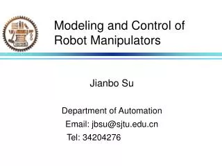
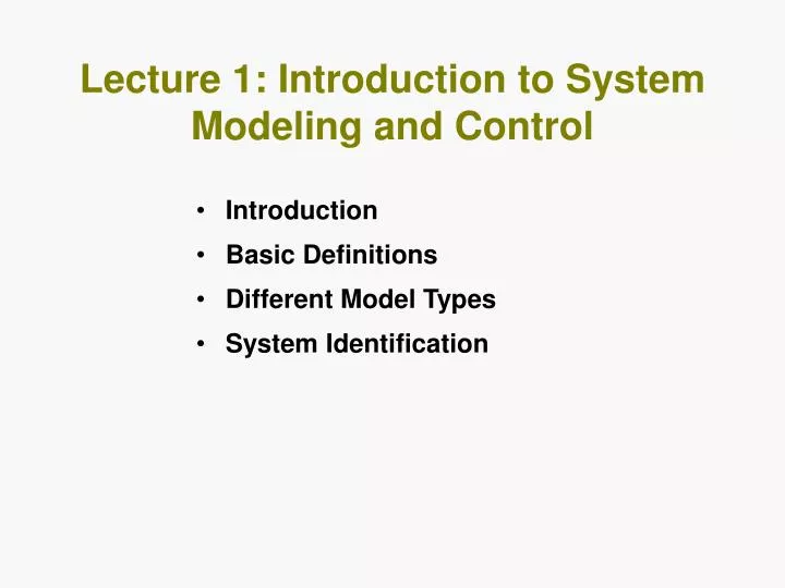
Lecture 1: Introduction to System Modeling and Control. Introduction Basic Definitions Different Model Types System Identification. What is Mathematical Model?. A set of mathematical equations (e.g., differential eqs.) that describes the input-output behavior of a system.

E N D
Lecture 1: Introduction to System Modeling and Control • Introduction • Basic Definitions • Different Model Types • System Identification
What is Mathematical Model? A set of mathematical equations (e.g., differential eqs.) that describes the input-output behavior of a system. What is a model used for? • Simulation • Prediction/Forecasting • Prognostics/Diagnostics • Design/Performance Evaluation • Control System Design
Definition of System System: An aggregation or assemblage of things so combined by man or nature to form an integral and complex whole. From engineering point of view, a system is defined as an interconnection of many components or functional units act together to perform a certain objective, e.g., automobile, machine tool, robot, aircraft, etc.
System Variables To every system there corresponds three sets of variables: Input variables originate outside the system and are not affected by what happens in the system Output variables are the internal variables that are used to monitor or regulate the system. They result from the interaction of the system with its environment and are influenced by the input variables y u System
y u M Dynamic Systems A system is said to be dynamic if its current output may depend on the past history as well as the present values of the input variables. Mathematically, Example: A moving mass Model: Force=Mass x Acceleration
Example of a Dynamic System Velocity-Force: Position-Force: Therefore, this is a dynamic system. If the drag force (bdx/dt) is included, then 2nd order ordinary differential equation (ODE)
Mathematical Modeling Basics Mathematical model of a real world system is derived using a combination of physical laws (1st principles) and/or experimental means • Physical laws are used to determine the model structure (linear or nonlinear) and order. • The parameters of the model are often estimated and/or validated experimentally. • Mathematical model of a dynamic system can often be expressed as a system of differential (difference in the case of discrete-time systems) equations
Different Types of Lumped-Parameter Models System Type Model Type Input-output differential or difference equation Nonlinear Linear State equations (system of 1st order eqs.) Linear Time Invariant Transfer function
Mathematical Modeling Basics • A nonlinear model is often linearized about a certain operating point • Model reduction (or approximation) may be needed to get a lumped-parameter (finite dimensional) model • Numerical values of the model parameters are often approximated from experimental data by curve fitting.
Linear Input-Output Models Differential Equations (Continuous-Time Systems) Inverse Discretization Discretization Difference Equations (Discrete-Time Systems)
u x x fs fs M M fd fd Example II: Accelerometer Consider the mass-spring-damper (may be used as accelerometer or seismograph) system shown below: Free-Body-Diagram fs(y): position dependent spring force, y=x-u fd(y): velocity dependent spring force Newton’s 2nd law Linearizaed model:
Example II: Delay Feedback Consider the digital system shown below: Input-Output Eq.: Equivalent to an integrator:
U G Y Transfer Function Transfer Function is the algebraic input-output relationship of a linear time-invariant system in the s (or z) domain Example: Accelerometer System Example: Digital Integrator Forward shift
Comments on TF • Transfer function is a property of the system independent from input-output signal • It is an algebraic representation of differential equations • Systems from different disciplines (e.g., mechanical and electrical) may have the same transfer function
Mixed Systems • Most systems in mechatronics are of the mixed type, e.g., electromechanical, hydromechanical, etc • Each subsystem within a mixed system can be modeled as single discipline system first • Power transformation among various subsystems are used to integrate them into the entire system • Overall mathematical model may be assembled into a system of equations, or a transfer function
Ra La B ia dc u J Electro-Mechanical Example Input: voltage u Output: Angular velocity Elecrical Subsystem (loop method): Mechanical Subsystem
Electro-Mechanical Example Power Transformation: Ra La B Torque-Current: Voltage-Speed: ia dc u where Kt: torque constant, Kb: velocity constant For an ideal motor Combing previous equations results in the following mathematical model:
Ra La B ia Kt u Transfer Function of Electromechanical Example Taking Laplace transform of the system’s differential equations with zero initial conditions gives: Eliminating Ia yields the input-output transfer function
B Reduced Order Model Assuming small inductance, La0 which is equivalent to • The D.C. motor provides an input torque and an additional damping effect known as back-emf damping
Brushless D.C. Motor • A brushless PMSM has a wound stator, a PM rotor assembly and a position sensor. • The combination of inner PM rotor and outer windings offers the advantages of • low rotor inertia • efficient heat dissipation, and • reduction of the motor size.
dq-Coordinates b q d e a e=p + 0 c offset Electrical angle Number of poles/2
Mathematical Model Where p=number of poles/2, Ke=back emf constant
System identification Experimental determination of system model. There are two methods of system identification: • Parametric Identification: The input-output model coefficients are estimated to “fit” the input-output data. • Frequency-Domain (non-parametric): The Bode diagram [G(jw) vs. w in log-log scale] is estimated directly form the input-output data. The input can either be a sweeping sinusoidal or random signal.
12 10 8 6 Amplitude 4 T 2 0 0 0.1 0.2 0.3 0.4 0.5 Time (secs) Electro-Mechanical Example Ra La Transfer Function, La=0: B ia Kt u u t k=10, T=0.1
Comments on First Order Identification • Graphical method is • difficult to optimize with noisy data and multiple data sets • only applicable to low order systems • difficult to automate
Least Squares Estimation Given a linear system with uniformly sampled input output data, (u(k),y(k)), then Least squares curve-fitting technique may be used to estimate the coefficients of the above model called ARMA (Auto Regressive Moving Average) model.
System Identification Structure Random Noise n Noise model Input: Random or deterministic Output plant y u • persistently exciting with as much power as possible; • uncorrelated with the disturbance • as long as possible
Basic Modeling Approaches • Analytical • Experimental • Time response analysis (e.g., step, impulse) • Parametric • ARX, ARMAX • Box-Jenkins • State-Space • Nonparametric or Frequency based • Spectral Analysis (SPA) • Emperical Transfer Function Analysis (ETFE)
20 10 Gain dB 0 -10 -1 0 1 2 10 10 10 10 1/T Frequency (rad/sec) 0 -30 Phase deg -60 -90 -1 0 1 2 10 10 10 10 Frequency (rad/sec) Frequency Domain Identification Bode Diagram of
Identification Data Method I (Sweeping Sinusoidal): f Ao Ai system t>>0 Method II (Random Input): system Transfer function is determined by analyzing the spectrum of the input and output
Random Input Method • Pointwise Estimation: This often results in a very nonsmooth frequency response because of data truncation and noise. • Spectral estimation: uses “smoothed” sample estimators based on input-output covariance and crosscovariance. The smoothing process reduces variability at the expense of adding bias to the estimate
System Models high order low order
Nonlinear System Modeling& Control Neural Network Approach
Real world nonlinear systems often difficult to characterize by first principle modeling First principle models are oftensuitable for control design Modeling often accomplished with input-output maps of experimental data from the system Neural networks provide a powerful tool for data-driven modeling of nonlinear systems Introduction
What is a Neural Network? • Artificial Neural Networks (ANN) are massively parallel computational machines (program or hardware) patterned after biological neural nets. • ANN’s are used in a wide array of applications requiring reasoning/information processing including • pattern recognition/classification • monitoring/diagnostics • system identification & control • forecasting • optimization
Benefits of ANN’s • Learning from examples rather than “hard” programming • Ability to deal with unknown or uncertain situations • Parallel architecture; fast processing if implemented in hardware • Adaptability • Fault tolerance and redundancy
Disadvantages of ANN’s • Hard to design • Unpredictable behavior • Slow Training • “Curse” of dimensionality
Biological Neural Nets • A neuron is a building block of biological networks • A single cell neuron consists of the cell body (soma), dendrites, and axon. • The dendrites receive signals from axons of other neurons. • The pathway between neurons is synapse with variable strength
Artificial Neural Networks • They are used to learn a given input-output relationship from input-output data (exemplars). • Most popular ANNs: • Multilayer perceptron • Radial basis function • CMAC
Input-Output (i.e., Function) Approximation Methods • Objective: Find a finite-dimensional representation of a function with compact domain • Classical Techniques • -Polynomial, Trigonometric, Splines • Modern Techniques • -Neural Nets, Fuzzy-Logic, Wavelets, etc.
Multilayer Perceptron • MLP is used to learn, store, and produce input output relationships x1 y x2 Training: network are adjusted to match a set of known input-output (x,y) training data Recall: produces an output according to the learned weights
Mathematical Representation of MLP y x W0 Wp Wk,ij: Weight from node i in layer k-1 to node j in layer k : Activation function, e.g., p: number of hidden layers
Universal Approximation Theorem (UAT) A single hidden layer perceptron network with a sufficiently large number of neurons can approximate any continuous function arbitrarily close. • Comments: • The UAT does not say how large the network should be • Optimal design and training may be difficult
Training Objective: Given a set of training input-output data (x,yt) FIND the network weights that minimize the expected error Steepest Descent Method: Adjust weights in the direction of steepest descent of L to make dL as negative as possible.
Neural Networks with Local Basis Functions These networks employ basis (or activation) functions that exist locally, i.e., they are activated only by a certain type of stimuli • Examples: • Cerebellar Model Articulation Controller (CMAC, Albus) • B-Spline CMAC • Radial Basis Functions • Nodal Link Perceptron Network (NLPN, Sadegh)
Biological Underpinnings • Cerebellum: Responsible for complex voluntary movement and balance in humans • Purkinje cells incerebellar cortex is believed to have CMAC like architecture
General Representation wi y x weights basis function • One hidden layer only • Local basis functions have adjustable parameters (vi’s) • Each weight wi is directly related to the value of function at some x=xi • similar to spline approximation • Training algorithms similar to MLPs