Download
1 / 26
290 likes | 573 Vues
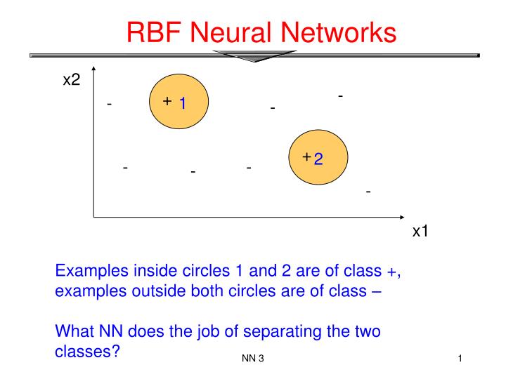
RBF Neural Networks. x2. -. +. -. 1. -. +. 2. -. -. -. -. x1. Examples inside circles 1 and 2 are of class +, examples outside both circles are of class – What NN does the job of separating the two classes?. Example 1.

E N D
RBF Neural Networks x2 - + - 1 - + 2 - - - - x1 Examples inside circles 1 and 2 are of class +, examples outside both circles are of class – What NN does the job of separating the two classes? NN 3
Example 1 Let t1,t2 and r1, r2 be the center and radius of circles 1 and 2, respectively, x = (x1,x2) example _t1 x1 1 y x2 _t2 1 _t1(x) = 1 if distance of x from t1 less than r1 and 0 otherwise _t2(x) = 1 if distance of x from t2 less than r2 and 0 otherwise Hyperspheric radial basis function NN 3
Example 1 _t2 - + - 2 - (0,1) + 1 - - - - _t1 (0,0) (1,0) Geometrically: examples are mapped to the feature space (_t1, _t2): examples in circle 2 are mapped to (0,1), examples in circle 1 are mapped to (1,0), and examples outside both circles are mapped to (0,0). The two classes become linearly separable in the (_t1, _t2) feature space! NN 3
x1 w1 x2 y wm1 xm RBF ARCHITECTURE • One hidden layer with RBF activation functions • Output layer with linear activation function. NN 3
Other Types of φ • Inversemultiquadrics • Gaussianfunctions (most used) NN 3
center Small Large Gaussian RBF φ φ : is a measure of how spread the curve is: NN 3
HIDDEN NEURON MODEL • Hidden units: use radial basis functions the output depends on the distance of the input x from the center t φ( || x - t||) x1 φ( || x - t||) t is called center is called spread center and spread are parameters x2 xm NN 3
Hidden Neurons • A hidden neuron is more sensitive to data points near its center. • For Gaussian RBF this sensitivity may be tuned by adjusting the spread , where a larger spread impliesless sensitivity. NN 3
x2 (0,1) (1,1) 0 1 y x1 (0,0) (1,0) Example: the XOR problem • Input space: • Output space: • Construct an RBF pattern classifier such that: (0,0) and (1,1) are mapped to 0, class C1 (1,0) and (0,1) are mapped to 1, class C2 NN 3
φ2 (0,0) Decision boundary 1.0 0.5 (1,1) 1.0 φ1 0.5 (0,1) and (1,0) Example: the XOR problem • In the feature (hidden layer) space: • When mapped into the feature space < 1 , 2 > (hidden layer), C1 and C2become linearly separable. Soa linear classifier with 1(x) and 2(x) as inputs can be used to solve the XOR problem. NN 3
x1 t1 -1 y x2 t2 -1 +1 RBF NN for the XOR problem NN 3
Application: FACE RECOGNITION • The problem: • Face recognition of persons of a known group in an indoor environment. • The approach: • Learn face classes over a wide range of poses using an RBF network. • See the PhD thesis by Jonathan Howell http://www.cogs.susx.ac.uk/users/jonh/index.html NN 3
Dataset • Sussex database (university of Sussex) • 100 images of 10 people (8-bit grayscale, resolution 384 x 287) • for each individual, 10 images of head in different pose from face-on to profile • Designed to good performance of face recognition techniques when pose variations occur NN 3
Datasets (Sussex) All ten images for classes 0-3 from the Sussex database, nose-centred and subsampled to 25x25 before preprocessing NN 3
RBF: parameters to learn • What do we have to learn for a RBF NN with a given architecture? • The centersof theRBF activation functions • the spreads of the Gaussian RBF activation functions • the weights from the hidden to the output layer • Different learning algorithms may be used for learning the RBF network parameters. We describe three possible methods for learning centers, spreads and weights. NN 3
Learning Algorithm 1 • Centers: are selected at random • centers are chosen randomly from the training set • Spreads: are chosen by normalization: • Then the activation function of hidden neuron becomes: NN 3
Learning Algorithm 1 • Weights:are computed by means of the pseudo-inverse method. • For an example consider the output of the network • We would like for each example, that is NN 3
Learning Algorithm 1 • This can be re-written in matrix form for one example and for all the examples at the same time NN 3
Learning Algorithm 1 let then we can write If is the pseudo-inverse of the matrix we obtain the weights using the following formula NN 3
Learning Algorithm 2: Centers • clustering algorithm for finding the centers • Initialization: tk(0) random k = 1, …, m1 • Sampling: draw x from input space • Similaritymatching: find index of center closer to x • Updating: adjust centers • Continuation: increment n by 1, goto 2 and continue until no noticeable changes of centers occur NN 3
Learning Algorithm 2: summary • Hybrid Learning Process: • Clustering for finding the centers. • Spreads chosen by normalization. • LMS algorithm for finding the weights. NN 3
Learning Algorithm 3 • Apply the gradient descent method for finding centers, spread and weights, by minimizing the (instantaneous) squared error • Update for: centers spread weights NN 3
Comparison with FF NN RBF-Networks are used for regression and for performing complex (non-linear) pattern classification tasks. Comparison between RBFnetworks and FFNN: • Both are examples of non-linear layered feed-forward networks. • Both are universal approximators. NN 3
Comparison with multilayer NN • Architecture: • RBF networks have one single hidden layer. • FFNN networks may have more hidden layers. • Neuron Model: • In RBF the neuron model of the hidden neurons is different from the one of the output nodes. • Typically in FFNN hidden and output neurons share a common neuron model. • The hidden layer of RBF is non-linear, the output layer of RBF is linear. • Hidden and output layers of FFNN are usually non-linear. NN 3
Comparison with multilayer NN • Activation functions: • The argument of activation function of each hidden neuron in a RBF NN computes the Euclidean distance between input vector and the center of that unit. • The argument of the activation function of each hidden neuron in a FFNN computes the inner product of input vector and the synaptic weight vector of that neuron. • Approximation: • RBF NN using Gaussian functions construct local approximations to non-linear I/O mapping. • FF NN construct global approximations to non-linear I/O mapping. NN 3