Download
1 / 79
810 likes | 1.26k Vues
Managing Business Process Flows:. Managing Flow Variability: Process Control and Capability. Managing Flow Variability. 9.1 Performance Variability 9.2 Analysis of Variability 9.3 Process Control 9.4 Process Capability 9.5 Process Capability Improvement 9.6 Product and Process Design.

E N D
Managing Business Process Flows: • Managing Flow Variability: Process Control and Capability
Managing Flow Variability • 9.1 Performance Variability • 9.2 Analysis of Variability • 9.3 Process Control • 9.4 Process Capability • 9.5 Process Capability Improvement • 9.6 Product and Process Design
Great year……. Great Products! Service! Reputation! Sorry to burst the bubble... But we are not doing well. Congratulations!! Good Job everyone! You’re Fired Yikes…more work We need to identify, correct and prevent future problems! I heard customers are not satisfied with our products and services Hhhmmm… we need hard data. Managing Business Process Flows:
Managing Business Process Flows: All Products & Services VARY in Terms Of Cost Quality Availability Flow Times Variability often leads to Customer Dissatisfaction Chapter covers some geographical/statistical methods for measuring, analyzing, controlling & reducing variability in product & process performance to improve customer satisfaction
§ 9.1 Performance Variability • All measures of product & process performance (external & internal) display Variability. • External Measurements - customer satisfaction, relative product rankings, customer complaints (vary from one market survey to the next) • Possible sources: supplier delivery delays or changing tastes • Internally - flow units in all business processes vary with respect to cost, quality & flow times • Possible sources: untrained workers or imprecise equipment Example 1 ~ No two cars rolling off an assembly line are identical. Even under identical circumstances, the time & cost required to produce the same product could be quite different. Example 2 ~ Cost of operating a department within a company can vary from one quarter to the next.
§ 9.1 Performance Variability • Variability refers to a discrepancy between the actual and the expected performance. • Can be due to gap between the following: • What customer wants and what product is designed for • What product design calls for and what process for making it is capable of producing • What process is capable of producing and what it actually produces • How the produced product is expected to perform and how it actually performs • How the product actually performs and how the customer perceives it • This often leads to: • higher costs, longer flow times, lower quality & DISSATISFIED CUSTOMERS
§ 9.1 Performance Variability • Processes with greater performance variability are generally judged LESS satisfactory than those with consistent, predictable performance. • Variability in product & process performance, not just its average, Matters to consumers! • Customers perceive any variation in their product or service from what they expected as a LOSS IN VALUE. • In general, a product is classified as defective if its cost, quality, availability or flow time differ significantly from their expected values, leading to dissatisfied customers.
Quality Management Terms BOOK COVERS A FEW QUALITY MANAGEMENT TERMS: • Quality of Design: how well product specifications aim to meet customer requirements (what we promise consumers ~ in terms of what the product can do) • Quality Function Deployment (QFD): conceptual framework for translating customers’ functional requirements (such as ease of operation of a door or its durability) into concrete design specifications (such as the door weight should be between 75 and 85 kg.) • Quality of conformance: how closely the actual product conforms to the chosen design specifications (how well we keep our promise in terms of how it actually performs) • Measures: fraction of output that meets specifications, # defects per car, percentage of flights delayed for more than 15 minutes OR the number of reservation errors made in a specific period of time.
§ 9.2 Analysis of Variability • To analyze and improve variability there are diagnostic tools to help us: • Monitor the actual process performance over time • Analyze variability in the process • Uncover root causes • Eliminate those causes • Prevent them from recurring in the future • Again we will use MBPF Inc. as an example and look at how their customers perceive the experience of doing business with the company & how it can be improved. • Need to present raw data in a way to make sense of the numbers, track change over time, or identify key characteristics of the data set.
§ 9.2.1 Check Sheets • A check sheet is simply a tally of the types and frequency of problems with a product or a service experienced by customers.
Check Sheets Pros • Easy to collect data Cons • Not very enlightening • No numerical characteristics
§ 9.2.2 Pareto Charts • A Pareto chart is simply a bar chart that plots frequencies of occurrences of problem types in decreasing order. • The 80-20 Pareto principle states that 20% of problem types account for 80% of all occurrences.
Pareto Charts Pros • Ranks problems • Shows relative size of quantities Cons • No numerical characteristics • Only categorizes data • No comparison process information
§ 9.2.3 Histograms • A histogram is a bar plot that displays the frequency distribution of an observed performance characteristic.
Histograms Pros • Visualizes data distribution • Shows relative size of quantities Cons • No numerical characteristics • Dependant on category size • No focus on change over time
Raw Data Pros • Actual information • Specific numbers Cons • Not intuitive • Does not help with understanding of relationships
§ 9.2.4 Run Charts • A run chart is a plot of some measure of process performance monitored over time • Advantage is that it is dynamic
Run Charts Pros • Shows data in chronological order • Displays relative change over time (trends, seasonality) Cons • Erratic graph • No numerical characteristics
§ 9.2.5 Multi-Vari Charts • A multi-vari chart is a plot of high-average-low values of performance measurement sampled over time.
Multi-Vari Charts Pros • Shows numerical range and average • Displays relative change over time Cons • Erratic graph • No numerical characteristics • Lacks distribution information • Does not provide guidance for taking actions
§ 9.3 Process Control • Goal Actual Performance vs. Planned Performance • Involves • Tracking Deviations • Taking Corrective Actions • Principle of feedback control of dynamical systems
Plan-Do-Check-Act (PDCA) • Process planning and process control are similar to the Plan-Do-Check-Act (PDCA) cycle. • PDCA cycle… • “involves planning the process, operating it, inspecting its output, and adjusting it in light of the observation.” • Performed continuously to monitor and improve the process performance • Main Problems • When to Act …. • Variances beyond control …
Process Control • Two types of variability • Normal variability • Statistically predictable • Structural variability and stochastic variability • Variations due to random causes only (worker cannot control) • PROCESS IS IN CONTROL • Process design improvement 2. Abnormal variability • Unpredictable • Disturbs state of statistical equilibrium of the process • Identifiable and can be removed (worker can control) • Abnormal - due to assignable causes • PROCESS IS OUT OF CONTROL
When is observed variability normal and abnormal??? Process Control • The short run goal is: • Estimate normal stochastic variability. • Accept it as an inevitable and avoid tampering • Detect presence of abnormal variability • Identify and eliminate its sources • The long run goal is to reduce normal variability by improving process.
§ 9.3.3 Control Limit Policy • Control Limit Policy • Control band • Range within variation in performance normal • Due to causes that cannot be identified or eliminated in short run • Leave alone and do not tamper • Variability outside this range is abnormal • Due to assignable causes • Investigate and correct • Applications • Inventory, Process Flow • Cash management • Stock trading
Process Control Chart: 9.3.4 Control Charts … Continued • - expected value of the performance • UCL and LCL • Standard Deviation • Assign z LCL = - z UCL = + z The smaller the value of “z”, the tighter the control
9.3.4 Control Charts … Continued • Within the control band Performance variability is normal • Outside the control band Process is “out of control” • Data Misinterpretation Type I error, : Process is “in control”, but data outside the Control Band Type II error, : Process is “out of control”, but data inside the Control Band
Optimal Degree of Control 9.3.4 Control Charts … Continued Acceptable Frequency “z” too small unnecessary investigation; additional cost “z” to large accept more variations, less costly In practice, a value of z = 3 is used 99.73% of all measurements will fall within the “normal” range
Take it one step further: Estimate by the overall average of all the sample averages, A A = (A1+ A2+…+AN) / N (N = # of samples) Also estimate by the standard deviation of all N x n observations, S 9.3.4 Control Charts … Continued • Average and Variation Control Charts • To calculate: Calculate the average value, A1, A2….AN Calculate the variance of each sample, V1, V2….VN A = /n (n = sample size) LCL = - z/n and UCL = + z/n
Average and Variation Control Charts 9.3.4 Control Charts … Continued New, Improved equations for UCL and LCL are: LCL = A - zs/n and UCL = A + zs/n Sample Variances CalculateV -- the average variance of the sample variances V = (V1+ V2+…+VN) / N (N = # of samples) Also calculate SV -- the standard deviation of the variances Variance Control Limits LCL = V - z sV and UCL = V + z sV If fall within this range Process Variability is stable If not within this range Investigate cause of abnormal variations
9.3.4 Control Charts … Continued • Average and Variation Control Charts Garage Door Example revisited… Ex: A1= (81 + 73 + 85 + 90 + 80) / 5 = 81.8 kg Ex: V1= (90 - 73) = 17 kg
A = 82.5 kg V = 10.1 kg Std. Dev. of Door Weights: s = 4.2 kg Std. Dev. of Sample Variances: sV = 3.5 kg 9.3.4 Control Charts … Continued • Average and Variation Control Charts Average Weights of Garage Door Samples:
9.3.4 Control Charts … Continued • Average and Variation Control Charts Let z = 3 Sample Averages UCL = A + zs/n = 82.5 + 3 (4.2) / 5 = 88.13 LCL = A - zs/n = 82.5 – 3 (4.2) / 5 = 76.87 Process is Stable!
9.3.4 Control Charts … Continued • Average and Variation Control Charts Let z = 3 Sample Variances UCL = V + z sV = 10.1 + 3 (3.5) = 20.6 LCL = V - zs sV = 10.1 – 3 (3.5) = - 0.4
9.3.4 Control Charts … Continued • Extensions Continuous Variables - Garage Door Weights, Processing Costs, Customer Waiting Time Use Normal distribution Discrete Variables - Number of Customer Complaints, Whether a Flow Unit is Defective, Number of Defects per Flow Unit Produced Use Binomial or Poisson distribution Control Limit formula differs, but basic principles is same.
9.3.5 Cause-Effect Diagrams • Cause-Effect Diagrams Sample Observations Plot Control Charts Abnormal Variability !! Now what?!! Brainstorm Session!! Answer 5 “WHY” Questions !
9.3.5 Cause-Effect Diagrams … Continued • Why…? Why…? Why…? Our famous “Garage Door” Example:
9.3.5 Cause-Effect Diagrams … Continued • Fishbone Diagram
9.3.6 Scatter Plots • The Thickness of the Sheet Metals Change Settings on Rollers Measure the Weight of the Garage Doors Determine Relationship between the two Plot the results on a graph: Scatter Plot
9.3 Section Summary • Process Control involves • Dynamic Monitoring • Ensure variability in performance is due to normal random causes only • Detect abnormal variability and eliminate root causes
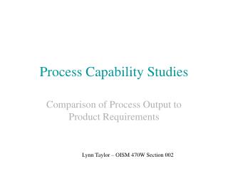
9.4 Process Capability • Ease of external product measures (door operations and durability) and internal measures (door weight) • Product specification limits vs. process control limits • Individual units, NOT sample averages - must meet customer specifications. • Once process is in control, then the estimates of μ (82.5kg) and σ (4.2k) are reliable. Hence we can estimate the process capabilities. • Process capabilities - the ability of the process to meet customer specifications • Three measures of process capabilities: • 9.4.1 Fraction of Output within Specifications • 9.4.2 Process Capability Ratios (Cpk and Cp) • 9.4.3 Six-Sigma Capability
9.4.1 Fraction of Output within Specifications • To compute for fraction of process that meets customer specs: • Actual observation (see Histogram, Fig 9.3) • Using theoretical probability distribution Ex. 9.7: • US: 85kg; LS: 75 kg (the range of performance variation that customer is willing to accept) See figure 9.3 Histogram: In an observation of 100 samples, the process is 74% capable of meeting customer requirements, and 26% defectives!!! OR: • Let W (door weight): normal random variable with mean = 82.5 kg and standard deviation at 4.2 kg, Then the proportion of door falling within the specified limits is: Prob (75 ≤ W ≤ 85) = Prob (W ≤ 85) - Prob (W ≤ 75)
9.4.1 Fraction of Output within Specifications cont… • Let Z = standard normal variable with μ = 0 and σ = 1, we can use the standard normal table in Appendix II to compute: AT US: Prob (W≤ 85) in terms of: Z = (W-μ)/ σ As Prob [Z≤ (85-82.5)/4.2] = Prob (Z≤.5952) = .724 (see Appendix II) (In Excel: Prob (W ≤ 85) = NORMDIST (85,82.5,4.2,True) = .724158) AT LS: Prob (W ≤ 75) = Prob (Z≤ (75-82.5)/4.2) = Prob (Z ≤ -1.79) = .0367 in Appendix II (In Excel: Prob (W ≤ 75) = NORMDIST(75,82.5,4.2,true) = .037073) THEN: Prob (75≤W≤85) = .724 - .0367 = .6873