Download
1 / 1
10 likes | 105 Vues
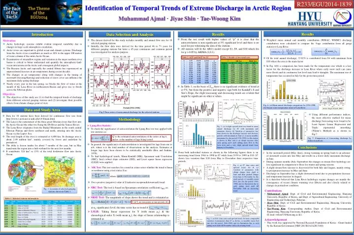
R233/EGU2014-1839. Identification of Temporal Trends of Extreme Discharge in Arctic Region. Muhammad Ajmal · Jiyae Shin · Tae- Woong Kim. Results. Results. Introduction. Data Selection and Analysis.

E N D
R233/EGU2014-1839 Identification of Temporal Trends of Extreme Discharge in Arctic Region Muhammad Ajmal· Jiyae Shin · Tae-Woong Kim Results Results Introduction Data Selection and Analysis • From the test result with higher values of “p” it is clear that the autocorrelation is non-significant at 5% significant level and there is no need for pre-whitening the data of the stations. • All stations will fit the AR(1) model except S1, S9, and S10 which fits for p > 0.05 by ARIMA (1,0,1). • Weighted mean annual and monthly contribution (WMAC, WMMC) discharge contribution were calculated to compare the %age contribution from all gauge stations to Lena River. • The dataset derived for this study includes monthly and annual flow rate for 10 selected gauging stations. • Initially, the flow data were derived for the time period 46 to 73 years for different gauging stations but latter a 45-year continuous and common period was investigated for analysis purpose. • Motivation • Arctic hydrologic systems exhibit evident temporal variability due to changes in large scale atmospheric circulation. • Arctic rivers are important to global ocean and climate systems. Discharge from the Arctic rivers contributes as much as 10% to the upper 100 meters of water column of the entire Arctic Ocean. • Examination of streamflow regime and variation in the major northern river basins is critical to better understand and quantify the atmospheric-land-ocean interactions in the Arctic and consequent global impacts. • The Russian Arctic and especially the central Siberia has experienced an unprecedented increase in air temperature during recent decades. • The changes in air temperature along with changes in the timing of snowmelt (freezing/thawing) and reduction of snow cover can influence the maximum daily spring discharge. • Nearly every year in the late spring, ice blocks the flow of water at the mouth of the Lena River in northeastern Russia and gives rise to floods across the Siberian plains. • at αL significance level, the time series has no trend if • LSLR:Taking linear regression for Y (with mean μy) & the chronological order X (with mean μx), the slope of linear relationship is estimated as Table 2: ACF and PACF for S5 Table 3: Results of two trend tests • Of the total annual discharge, 33.02% is contributed from S4 with minimum from S10 where the area is the main factor. • In Fig. 6(b) a comparison has been made for the temperature rise which is a key factor for the discharge increase in Lena River where early snow melt can cause more floods and its continuous low level may lead to draughts. The maximum rise of temperature has occurred in July for the given time period. (a) (b) • In Table 3, on the basis of Zcrit there is no significant evidence of trend at α=5%, but from the positive and negative sign both for Kendall’s S and Sen’s Slope, the slight increasing and decreasing trends are evident that might be significant on other α values. • Objectives • The objectives of this study are (1) to find the temporal trends of discharge from different selected gauging stations and (2) investigate their possible effects from climate change point of view. (a) (b) Fig. 6: (a) Mean annual discharge comparison for 1954-1998, (b) Stream water temperature trend of Lena River Data and Study Area Source: Yang D. & Liu B. (2005) Fig.2 Time series of mean annual discharge for the selected stations • Using different performance indices, the most effective method for mean discharge forecasting were found to be Least Square Linear Regression and Triple exponential smoothing (Winter’s Method) as is shown in Fig.7. • Data for 10 stations have been derived for continuous flow rate from http://www.r-arcticnet.sr.unh.edu/v4.0/main.html. • The Lena is the easternmost of the three great Siberian rivers that flow into the Arctic Ocean (the other two being the Ob River and the Yenisei River). • The Lena River originates from the Baikal Mountains in the south central Siberian Plateau and flows northeast and north, entering into the Arctic Ocean via the Laptev Sea. • The total length of the river is estimated at 4,400 km. Its drainage area is about 2.49 million km2, mainly covered by forest and underlain by permafrost. • The delta is frozen tundra for about 7 months of the year, but in May transforms the region into a lush wetland for the next few months. • It contributes 524 km3 or 15% of the total freshwater flow into Arctic Ocean. Methodology • Ljung-Box Statistic: • To check the significance of autocorrelation the Ljung-Box test was applied with test statistics as: (c) Fig. 3: (a) A slight upward trend was found in mean annual discharge for S3 with maximum and minimum shown. (b) Variation of parameters has been shown for the discharge increase and decrease periods with maximum in June (c) A mean monthly maximum (for the period 1936-1999) for this station is shown in May and is an abrupt increase after early spring snow melt adding more flow to the Leva river and a very slight upward trend from January to December. • is the estimated autocorrelation of the series at lagk, and m is the number of lags being tested. Fig. 7: Comparison of forecasting discharge by different methods • In general, the significance of autocorrelation is investigated for lags from one to n/4, where n is the total number of observations in the analysis. Estimates at longer lags have been shown to be statistically unreliable (Box and Jenkins, 1970). • To find hydrological trends, Mann-Kendall (MK), Spearman rank Correlation (SRC), Sen’s robust slope estimator (SSE), and Least square linear regression (LSLR) were applied. Conclusions • From both individual stations as shown in the following figures there is an increasing trend from 1944 to 1998 in S7 while from 1939 to 1999 in S10. S7 shows less variation than S10 from May to December their respective time periods. • In the snowmelt period (May–June), strong warming in spring leads to an advance of snowmelt season into late May and results in a lower daily maximum discharge in June. • During summer months (July–September) the changes in stream flow hydrology are less significant in comparison to those for winter and spring seasons. • A slight stream flow increase is discovered for both July and August, mainly owing to precipitation increase in May and June. • Discharge in September has a slight downward trend due to precipitation decrease and temperature increase in August. • It is therefore believed that Lena River hydrologic regime changes are mainly the consequence of recent climate warming over Siberia and also closely related to changes in permafrost condition. Fig. 4: (a) S7, time series and upward trend, (b) & (c) variation of parameters with abrupt change from April to June and then gradual change from June to November for the study period, (c) monthly mean flow rate (for the period 1944-1998) and its fluctuation due to early spring snow melt till November with an increasing trend. • MK Test: This test searches for a trend in a time series whether the trend is linear or nonlinear using a test statics S as: • where • For a positive (negative) value of S indicates an upward(downward) trend. (a) (b) (c) • SRC Test: The test is based on Spearman correlation coefficient rSRC as: • SRSE Test:The magnitude of slope shows the trend and is estimated as: Fig. 1: Location of selected gauging stations shown in Table 1 • Contributions • Muhammad Ajmal: Dept. of Civil and Environmental Engineering, Hanyang University, Republic of Korea, and Dept. of Agricultural Engineering, University of Engineering and Technology, Pakistan. • Jiyae Shin: Dept. of Civil and Environmental Engineering, Hanyang University, Republic of Korea. • Tae-Woong Kim: Corresponding Author, Dept. of Civil and Environmental Engineering, Hanyang University, Republic of Korea. • (E-mail: twkim72@hanyang.ac.kr). Table 1: Selected stations information (a) Yi & Yj are data points at time periods i & j (b) (c) Fig. 5: (a) S10, time series and upward trend, (b) more comparable variation of parameters than S7 as shown, (c) monthly mean flow rate (for the period 1944-1998) and its fluctuation due to early spring snow melt till November with a decreasing trend. • Acknowledgement • This work was supported by National Research Foundation of Korea - Grant funded by the Korean Government (NRF-2013R1A1A2013160)