Download
1 / 24
400 likes | 1.33k Vues
Introduction to Econometrics. Lecture 10 Simultaneous equations models. Single equations or systems of equations?. Even if we are only interested in one particular equation (e.g. a demand function or a consumption function) we may have to consider it as part of a system of equations.

E N D
Introduction to Econometrics Lecture 10 Simultaneous equations models
Single equations or systems of equations? Even if we are only interested in one particular equation (e.g. a demand function or a consumption function) we may have to consider it as part of a system of equations.
Endogenous regressors and bias • Bias. Single equation (OLS) estimators will be biased if one or more regressors is endogenous (jointly dependent). • Consistency. But other methods, such as Indirect Least Squares, Instrumental Variables or Two Stage Least Squares estimation, may be available to obtain consistent estimators.
The identification problem • Even before we worry about bias we must be sure that we can identify the equation of interest in the system.
Simultaneous equation model of an agricultural product In his textbook Bill Greene uses the following simple model of the agricultural sector to illustrate both these issues D and S are respectively measures of quantity demanded and supplied in the market P is a measure of the price of agricultural goods Y is a measure of consumers’ income u and v are unobservable stochastic disturbance terms
The condensed structural form of the model First, because we cannot separately observe D and S, let us simply replace them both by Q and condense the model to two equations. [1] [2] So we have a two equation model with two endogenous variables (Q,P) and one exogenous variable (Y). Unfortunately OLS estimation of the supply function would result in biased estimators for b0 and b1 (because P and v are not independent). It would also not be possible to obtain any sensible estimators for the demand function because it would not be identified.
The reduced form of the model The reduced form of a model expresses each endogenous variable only in terms of the exogenous variable(s). So here we might have [3] [4] We could use OLS to obtained unbiased estimates of the parameters. The supply equation is identified because it is possible to solve for the b parameters in equation [2] in terms of the s . (See later slide for proof). The demand equation is not identified because it is not possible to solve for the as in in equation [1] terms of the s.
Detail on the reduced form equation for P Equating (1) and (2) and rearranging we can get the price reduced form equation. So we can see the following relationships between the s and the bs
Detail on the reduced form equation for Q Now substitute this back into equation [1] Collecting terms together and tidying up we find So we can see the following relationships between the s and the as
Solving for the b parameters Structural form parameters are identified if we can solve for them algebraically using information about the reduced from parameters. We can now see that which just reduces to b1 The method of Indirect Least Squares (which is suitable for an exactly identified equation like the supply equation here) can be used to get structural form Parameter estimates indirectly. First estimate the reduce from, then solve for the structural form parameters mathematically. However this method does not provide standard errors for the structural form parameter estimates. As we shall see later the Two Stage Least Squares/Instrumental Variables approach to estimation can do this for us. These estimators, although biased, are consistent.
Identification • An equation is under-identified (or not identified) if its structural (behavioural) parameters cannot be expressed in terms of the reduced form parameters. • An equation is exactly identified if its structural (behavioural) parameters can be uniquely expressed in terms of the reduced form parameters. • An equation is over-identified if there is more than one solution for expressing its structural (behavioural) parameters in terms of the reduced • form parameters. • Here the supply equation is exactly identified but the demand function is not identified.
Identification conditions • A system of G equations (containing G endogenous variables) must exclude at least G-1 variables from a given equation in order for the parameters of that equation to be identified and to be able to be consistently estimated. • So we can confirm that the supply equation in our model is exactly identified as here G=2. • The supply equation excludes G-1 = 1 variable (Y) and so the condition is exactly satisfied. • The demand equation excludes none of the variables in the model – the condition is not satisfied. The demand equation is not identified.
Graphical illustration of the identification of the supply equation The points cluster around the supply curve due to shifts in demand as Y varies.
Simultaneous equation bias OLS estimation of equation 2 will be biased because P and v are not statistically independent i.e. E(Pv)0 Proof Now since
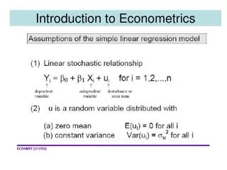
In a single equation regression model we require E(u|X) = E(u) (which is = 0 by assumption) u must be independent of each X. • If this condition is not satisfied then OLS estimators will be biased (proof on next two slides). • There are several ways that this assumption might be violated: • endogenous regressors (the equation is part of a simultaneous equation model and one of the regressors is endogenous (jointly determined) – simultaneous equation bias • there is an omitted variable that is correlated with one of the included variables • one or more of the X variables has systematic measurement errors such that the observed values are not independent of the disturbance Bias more generally
Instrumental variables estimation If a regressor (such as P) is not independent of the disturbance term we might nevertheless be able to replace it by another variable (instrumental variable) that is • highly correlated with P • but uncorrelated with the disturbance term If such a variable was to be available we could estimate the supply equation using Instrumental Variables (IV) estimation. Instrumental Variables estimators, although biased, are consistent.
Finding a suitable Instrumental Variable • How do we find an instrumental variable? • There are two methods: • Arbitrary search and test. • Two stage least squares. • Two Stage Least Squares (2SLS) offers an excellent direct estimation method in the case of exactly or over-identified equations.
Two stage least squares (2SLS) • While it is still a single equationestimation technique, 2SLS uses the information available from the specification of the entire equation system. • In doing so, it is able to provideunique estimates of each structural parameter in the over-identified equation.
Two stage least squares as IV estimation • The first stage involves the creation of an instrument. Use the reduced from equation for P to get its fitted value, Phat. • The second stage involves a variant of instrumental variables estimation. Replace P by Phat in the supply equation and use OLS in this second stage of the estimation process • So it is in fact a special way and perhaps less arbitrary way of doing instrumental variables estimation.
Two stage least squares estimation with modern econometric software • Although one could undertake 2SLS estimation manually, running the reduced form regression, saving the fitted values and then running the second stage (structural form) regression, modern software allows you to get the results automatically with one set of instructions. • You need to tell the software which RHS variable is endogenous and which other variables should be used as regressors in the reduced form (first stage) of the regression. • Using the automatic IV procedure will also guarantee appropriate estimates of the second stage standard errors.
PcGive automates the two stage least squares (instrumental variables) estimation procedure – and provides appropriate estimates of the second stage standard errors The screen grab below shows how I formulated the IV estimation for my equation. The first endogenous variable listed is used on the LHS (i.e. Q). The second endogenous variable (P) is fitted to the “reduced form” equation with Income marked as an instrument. You “right-click” on variables in the left-hand pane to change their status. Instrumental variables estimation in PcGive
Results Using yearly data on price and quantity for the US agricultural sector and real personal disposable income for US consumers for the years 1960 to 1986 Greene (2000) estimates the supply equation both by OLS and instrumental variables estimation. EQ( 1) Modelling Q by OLS (using agsupply.xls) The estimation sample is: 1960 - 1986 Coefficient Std.Error t-value t-prob Part.R^2 Constant 54.1320 4.526 12.0 0.000 0.8512 P 0.419530 0.04959 8.46 0.000 0.7411 sigma 8.29028 RSS 1718.22044 R^2 0.741113 F(1,25) = 71.57 [0.000]** log-likelihood -94.3796 DW 1.68 no. of observations 27 no. of parameters 2 mean(Q) 89.963 var(Q) 245.813 EQ( 2) Modelling Q by IVE (using agsupply.xls) The estimation sample is: 1960 - 1986 Coefficient Std.Error t-value t-prob P Y 0.503798 0.06006 8.39 0.000 Constant 46.9349 5.399 8.69 0.000 sigma 8.75596 RSS 1916.66914 Reduced form sigma 7.0498 no. of observations 27 no. of parameters 2 no. endogenous variables 2 no. of instruments 2 mean(Q) 89.963 var(Q) 245.813 Additional instruments: [0] = Income Testing beta = 0: Chi^2(1) = 70.363 [0.0000]**