Download
1 / 30
360 likes | 747 Vues
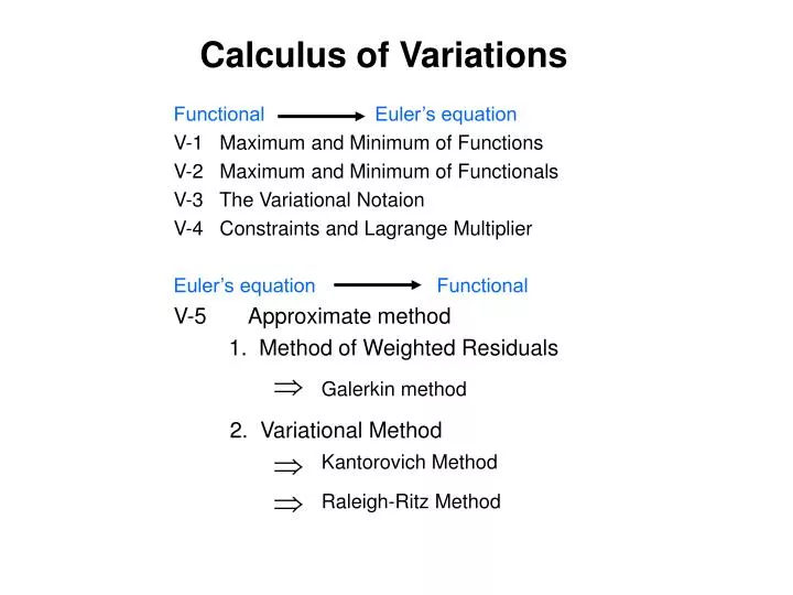
Calculus of Variations. Functional Euler’s equation V-1 Maximum and Minimum of Functions V-2 Maximum and Minimum of Functionals V-3 The Variational Notaion V-4 Constraints and Lagrange Multiplier Euler’s equation Functional

E N D
Calculus of Variations Functional Euler’s equation V-1 Maximum and Minimum of Functions V-2 Maximum and Minimum of Functionals V-3 The Variational Notaion V-4 Constraints and Lagrange Multiplier Euler’s equation Functional V-5 Approximate method 1. Method of WeightedResiduals Galerkin method 2. Variational Method Kantorovich Method Raleigh-Ritz Method
V-1 Maximum and Minimum of Functions Part A Functional Euler’s equation Maximum and Minimum of functions (a)If f(x) is twice continuously differentiable on [x0 , x1] i.e. Nec. Condition for a max. (min.) of f(x) at is that Suff. Condition for a max (min.) off(x) at are that also ( ) (b)If f(x) over closed domain D. Then nec. and suff. Condition for a max. (min.) i = 1,2…n and also that is a negative infinite . of f(x) at x0 are that
(c)If f(x) on closed domain D If we want to extremize f(x) subject to the constraints i=1,2,…k ( k < n ) Ex :Find the extrema of f(x,y) subject to g(x,y) =0 (i) 1st method : by direct diff. of g To extremize f
We have and to find (x0,y0) which is to extremize f subject to g = 0 (ii) 2nd method : (Lagrange Multiplier) extrema of v without any constraint extrema of f subject to g = 0 To extremize v Let We obtain the same equations to extrimizing. Where is called The Lagrange Multiplier.
V-2 Maximum and Minimum of Functionals y 2.1 What are functionals. Functional is function’s function. x 2.2 The simplest problem in calculus of variations. Determine such that the functional: where over its entire domain , subject to y(x0) = y0 , y(x1) = y1at the end points. as an extrema
On integrating by parts of the 2nd term ------- (1) since and since is arbitrary. -------- (2) Euler’s Equation Natural B.C’s or /and The above requirements are called national b.c’s.
V-3 The Variational Notation Variations Imbed u(x) in a “parameter family” of function the variation of u(x) is defined as The corresponding variation of F , δF to the order in ε is , since and Then
Thus a stationary function for a functional is one for which the first variation = 0. For the more general cases , • Several dependent variables. Ex : Euler’s Eq. (b) Several Independent variables. Ex : Euler’s Eq.
(C) High Order. Ex : Euler’s Eq. Variables Causing more equation. Order Causing longer equation.
V-4 Constraints and Lagrange Multiplier Lagrange multiplier • Lagrange multiplier can be used to find the extreme value of a multivariate function f subjected to the constraints. • Ex : • Find the extreme value of • ------------(1) • From -----------(2) where and subject to the constraints
Because of the constraints, we don’t get two Euler’s equations. From The above equations together with (1) are to be solved for u , v. So (2)
(b) Simple Isoparametric Problem To extremize , subject to the constraint: (1) (2) y (x1) = y1 , y (x2) = y2 Take the variation of two-parameter family: (whereand are some equations which satisfy ) Then , To base on Lagrange Multiplier Method we can get :
i = 1,2 So the Euler equation is: when , is arbitrary numbers. The constraint is trivial, we can ignore .
Examples Euler’s equation Functional Helmholtz Equation Ex : Force vibration of a membrane. -----(1) if the forcing function f is of the form we may write the steady state disp u in the form (1)
-----(2) Consider Note that
Hence : • if is given on • i.e. on • then the variational problem • -----(3) • (ii) if is given on • the variation problem is same as (3) • if is given on
Diffusion Equation Ex : Steady state Heat condition in D B.C’s : on B1 on B2 on B3 multiply the equation by , and integrate over the domain D. After integrating by parts, we find the variational problem as follow. with T = T1 on B1
Poison Equation Ex : Torsion of a primatri Bar in R on where is the Prandtl stress function and , The variation problem becomes with on
V-5-1 ApproximateMethods (I) Method of Weighted Residuals (MWR) in D +homo. b.c’s in B Assume approx. solution where each trialfunctionsatisfies the b.c’s The residual In this method (MWR), Ci are chosen such that Rn is forced to be zero in an average sense. i.e. < wj, Rn > = 0, j = 1,2,…,n where wj are the weighting functions..
(II)Galerkin Method wj are chosen to be the trial functions hence the trial functions is chosen as members of a complete set of functions. Galerkin method force the residual to be zero w.r.t. an orthogonal complete set. Ex: Torsion of a square shaft (i) one – term approximation
From therefore the torsional rigidity the exact value of D is the error is only -1.2%
(ii) two – term approximation By symmetry → even functions From and we obtain therefore the error is only -0.14%
V-5-2 Variational Methods (I) Kantorovich Method Assuming the approximate solution as : where Ui is a known function decided by b.c. condition. Euler Equation of Ci Ci is a unknown function decided by minimal “I”. Ex : The torsional problem with a functional “I”.
Assuming the one-term approximate solution as : Then, Integrate by y Euler’s equation is where b.c. condition is General solution is
where and So, the one-term approximate solution is
(II) Raleigh-Ritz Method This is used when the exact solution is impossible or difficult to obtain. First, we assume the approximate solution as : Where, Uiare some approximate function which satisfy the b.c’s. Then, we can calculate extreme I . choose c1 ~ cn i.e. Ex: , Sol : From
Assuming that (1)One-term approx (2)Two-term approx Then,
0.317 c1 + 0.127 c2 = 0.05 c1 = 0.177 , c2 = 0.173 ( It is noted that the deviation between the successive approxs. y(1) andy(2) is found to be smaller in magnitude than 0.009 over (0,1))