Download
1 / 32
320 likes | 488 Vues
Effort Estimation. For example?. Has been an “ art ” for a long time because many parameters to consider unclear of relative importance of the parameters unknown inter-relationship among the parameters unknown metrics for the parameters Historically , project managers

E N D
Effort Estimation For example? • Has been an “art” for a long time because • many parameters to consider • unclear of relative importance of the parameters • unknown inter-relationship among the parameters • unknown metrics for the parameters • Historically, project managers • consulted others with past experiences • drew analogy from projects with “similar” characteristics • broke the projects down to components and used past history of workers who have worked on similar components; then combined the estimates
Class Discussion of Size vs Effort Effort If the relation is non-linear then ---- ? Effort = a + b * (Size) Size
General Model • There have been many proposed models for estimation of effort in software. They all have a “similar” general form: Effort≡ (size) and (set of factors) • Effort = [a + (b * ((Size)**c))] * [PROD(f’s)] • where : • Size is the estimated size of the project in loc or function points • a, b, c, are coefficients derived from past data and curve fitting • a = base cost to do business regardless of size • b = fixed marginal cost per unit of change of size • c = nature of influence of size on cost • f’s are a set of additional factors, besides Size, that are deemd important • PROD (f’s) is the arithmetic-product of the f’s
COCOMO Estimating Technique • Developed by Barry Boehm in early 1980’s who had a long history with TRW and government projects (LOC based) • Later modified into COCOMO II in the mid-1990’s (FP preferred or LOC) • Assumed process activities : • Product Design • Detailed Design • Code and Unit Test • Integration and Test • Utilized by some but most of the people still rely on experience and/or own company proprietary data & process. (e.g. proprietary loc to pm conversion rate) Note that this does not includerequirements !
Basic Form for Effort • Effort = A * B * (size ** C) • or more “generally” • Effort = [A * (size**C)] * [B ] • Effort = person months • A = scaling coefficient • B = coefficient based on 15 parameters • C = a scaling factor for process • Size = delivered source lines of code in “KLOC”
Basic form for Time • Time = D * (Effort ** E) • Time = total number of calendar months • D = A constant scaling factor for schedule • E = a coefficient to describe the potential parallelism in managing software development
COCOMO I • Originally based on 56 projects • Reflecting 3 modes of projects • Organic: less complex and flexible process • Semidetached : average project • Embedded : complex, real-time defense projects
3 Modes are Based on 8 Characteristics • A. Team’s understanding of the project objective • B. Team’s experience with similar or related project • C. Project’s needs to conform with established requirements • D. Project’s needs to conform with established interfaces • E. Project developed with “new” operational environments • F. Project’s need for “new” technology, architecture, etc. • G. Project’s need for schedule integrity • H. Project’s “size” range
Understand require. Exp. w/similar project Conform w/req. Conform w/int. New oper. env. New tech/meth. Schedule int. Size
COCOMO I • For the basic forms: • Effort = A * B *(size)C • Time = D * (Effort)E • Organic : A = 3.2 ; C = 1.05 ; D= 2.5; E = .38 • Semidetached : A = 3.0 ; C= 1.12 ; D= 2.5; E = .35 • Embedded : A = 2.8 ; C = 1.20 ; D= 2.5; E = .32 What about the coefficient B? ---- see next slide
Coefficient B • Coefficient B is an effort adjustment factor based on 15 parameters which varied from very low,low,nominal, high, very high to extra high • B = product (15 parameters) • Product attributes: • Required Software Reliability : .75 ; .88; 1.00; 1.15; 1.40; • Database Size : ; .94; 1.00; 1.08; 1.16; • Product Complexity : .70 ; .85; 1.00; 1.15; 1.30; 1.65 • Computer Attributes • Execution Time Constraints : ; ; 1.00; 1.11; 1.30; 1.66 • Main Storage Constraints : ; ; 1.00; 1.06; 1.21; 1.56 • Virtual Machine Volatility : ; .87; 1.00; 1.15; 1.30; • Computer Turnaround time : ; .87; 1.00; 1.07; 1.15;
Coefficient B (cont.) • Personnel attributes • Analyst Capabilities : 1.46 ; 1.19; 1.00; .86; .71; • Application Experience : 1.29; 1.13; 1.00; .91; .82; • Programmer Capability : 1.42; 1.17; 1.00; .86; .70; • Virtual Machine Experience : 1.21; 1.10; 1.00; .90; ; • Programming lang. Exper. : 1.14; 1.07; 1.00; .95; ; • Project attributes • Use of Modern Practices : 1.24; 1.10; 1.00; .91; .82; • Use of Software Tools : 1.24; 1.10; 1.00; .91; .83; • Required Develop schedule : 1.23; 1.08; 1.00; 1.04; 1.10;
A “cooked up” example Any problem? • Consider an average project of 10Kloc: • Effort = 3.0 * B * (10** 1.12) = 3 * 1 * 13.2 = 39.6 pm • Where B = 1.0 (all nominal) • Time = 2.5 *( 39.6 **.35) = 2.5 * 3.6 = 9 months • This requires an additional 8% more effort and 36% more schedule time for product plan and requirements: • Effort = 39.6 + (39.6 * .o8) = 39.6 + 3.16 = 42.76 pm • Time = 9 + (9 * .36) = 9 +3.24 = 12.34 months
Try another example(how about your own project?) • Go through the assessment of 15 parameters for the effort adjustment factor, B. • You may have some concerns if your company adopts COCOMO : • Are we interpreting each parameter the same way • Do we have a consistent way to assess the range of values for each of the parameters • How do we get more accuracy in LOC estimate
Relative Accuracy of Estimates(from B. Boehm) 4x Estimate Range (size/cost) Actual size/cost x .25x Requirements Code/Test Design Early feasibility Stages of the Project
COCOMO II • Based on 2 major realizations: • Realizes that there are many different software life cycle and development models, while COCOMO I assumed waterfall type of model • Realizes that estimates depends on granularity of information --- the more information (later stage of development) the more accurate is the estimate Effort (nominal) = A * (size )C Effort (adjusted) = { A * (size )C } * B
COCOMO II • COCOMO research effort performed at USC with many industrial corporations participating – still lead by Barry Boehm • Has a database of over 80 some newer projects
COCOMO II emphasis • COCOMO II - Effort (nominal) = A * (size )C: • Removal of “modes”: Instead of the 3 “modes,” which use 8 characteristics to determine the modes, use 5 factors to determine the scaling coefficient, “C” • Precedentedness • Flexibility • Risk • Team cohesion • Process maturity • COCOMO II - Effort (adjusted) = A * (size )C * B : • For Early Estimate, preferred to use Function Pointinstead of LOC for size (loc is harder to estimate without some experience). Coefficient “B” rolled up to 7 cost drivers (1. prod reliability & complex; 2. reuse req.; 3. platform difficulty; 4. personnel; 5. personnel experience; 6 facility; 7. schedule) • ForPost-Architecture Estimates, may use either loc or function points. Coefficient “B” use 17 cost drivers, expanded form the 7 cost drivers (e.g. personnel expands into 1) analyst capability; 2) programmer capability, 3) personnel continuity)
Function Point • A non-LOC based estimator • Often used to assess software “complexity” and “size” • Started by Albrecht of IBM in late 1970’s
Function Point (product size/complexity) • Gained momentum in the 1990’s with IFPUG as software service industry looked for a metric • Function Point does provide some advantages over loc • language independent • don’t need the actual lines of code to do the counting • takes into account of different entities • Some disadvantages include : • complex to come up with the final number • consistency (data reliability) varies by people --- although IFPUG membership and training have improved on this
Function Point Metric via GQM* • Goal : Measure the Size of Software • Question: What is the size of a software in terms of its: • Data files • Transactions • Metrics: Function Points ---- (defined in this lecture) * GQM is a methodology invented and advocated by V. Basili of U. of Maryland
FP Utility • Where is FP used? • Comparing software in a “normalized fashion” independent of op. system, languages, etc. • Benchmarking and Projection based on “size”: • size -> cost or effort • size -> development schedule • size -> defect rate • Outsourcing Negotiation
Methodology(“extended version” --- compared to your text) Composed of 3 major steps: • Identify and Classifying: • Data • Transactions • Evaluation of Complexity Levels of Data and Transactions • Compute the Functional Point
1. Identifying & Classifying 5 “Basic Entities” • Data: • Internally generated and stored (logical files and tables) • Data maintained externally and requires an external interface to access (external interfaces) • Transactions: • Information or data entry into a system for transaction processing (inputs) • Information or data “leaving” the system such as reports or feeds to another application (outputs) • Information or data retrieved and displayed on the screen in response to query (query)
2. Evaluating Complexity • Using a complexity table, each of the 5 basic entities is evaluated as : • Low (simple) • Average • High (complex) • 3 attributes are used for the above complexity table decisions • # ofRecord Element Types (RET): e.g. employee data type, student record type • # of unique attributes (fields) or Data Element Types (DET) for each record : e.g. name, address, employee number, and hiring date would make 4 DETs for employee data stype • # ofFile Type Referenced (FTR): e.g an external payroll record file that needs to be accessed
5 Basic Entity Types uses the RET, DET, and FTRfor Complexity Evaluation For -- Internal Logical Files and External Interfacesdata entities: # of RET1-19 DET20-50 DET50+ DET 1 Low Low Ave 2 -5 Low Avg High 6+ Avg High High For -- Input, Output and Query transactions: # of FTR1-4 DET5 -15 DET16+ DET 0 - 1 Low Low Ave 2 Low Avg High 3+ Avg High High
Example • Consider a requirement: “has the feature to add a new employee to the “system.” • Assume employee information involves 3 external files that each has a different Record Element Types (RET) • Employee Basic Information has employee data records • Each employee record has 55 fields (1 RET and 55 DET) - AVERAGE • Employee Benefits records • Each benefit record has 10 fields (1 RET and 10 DET) - LOW • Employee Tax records • Each tax record has 5 fields ( 1 RET and 5 DET) - LOW • Adding a new employee involves 1 input transaction which involves 3 file types referenced (FTR) and a total of 70 fields (DET). So for the 1 input transaction the complexity is HIGH
Function Point (FP) Computation • Composed of 5 “Basic Entities” • input items (external input items from user or another application) • output items (external outputs such as reports, messages, screens – not each data item) • Queries (a query that results in a response of one or more data) • master and logical files (internal file or data structure or data table) • external interfaces (data or sets of data sent to external devices, applications, etc.) • And a “complexity level index” matrix : Simple(low) Complex (high) Average 3 4 6 Input 5 7 Output 4 3 Query 4 6 Logical files 7 10 15 Ext. Interface & file 7 5 10
Function Point Computation (cont.) • Initial Function Point : Σ [Basic Entity x Complexity Level Index] all basic entities Continuing the Example of adding new employee: - 1 external interface (average) = 7 - 1 external interface (low) = 5 - 1 external interface (low) = 5 - 1 input (high) = 6 Initial Function Point = 7 + 5 + 5 + 6 = 23 Note that ---- this just got us to Initial Function Point
Function Point Computation (cont.) • Initial Function Point : ∑ (Basic Entity x Complexity Level Index) is modified by 14 DI’s • There are 14 more “Degree of Influences” ( 0 to 5 scale) : • data communications • distributed data processing • performance criteria • heavy hardware utilization • high transaction rate • online data entry • end user efficiency • on-line update • complex computation • reusability • ease of installation • ease of operation • portability • maintainability These form the 14 DIs
Function Point Computation (cont.) • Define Technical Complexity Factor (TCF): • TCF = .65 + [(.01) x (14 DIs )] • where DI = ∑ ( influence factor value) • So note that .65 ≤ TCF ≤ 1.35 Function Point (FP) = Initial FP x TCF Finishing the earlier Example: for the example, assume TCF came out to be 1.15, then Function Point = 23 x 1.15 = 26.45
Function Point • Provides you another way to estimate the “size” of the project based on estimating 5 basic entities : • Inputs • Outputs • Logical Files • External Interfaces • Queries • (note : the text book algorithm is earlier, simplified version) (important) • ** Then --- still need to have an estimate on productivity e.g. function point/person-month • ***Divide the estimated total project function points (size) by the productivity to get an estimate of “effort” in person-month or person-days needed. - - - - - - - - - - - - - - - - - - - - - - - -