Download
1 / 87
880 likes | 1.05k Vues
Learn about the history and principles of chromatography, the various techniques including liquid chromatography, gas chromatography, and supercritical fluid chromatography, and how solutes are separated based on differential migration. Understand the concept of elution chromatography, chromatograms, retention times, and migration rates of solutes.

E N D
An Introduction to Chromatographic Separations It was Mikhail Tswett, a Russian botanist, in 1903 who first invented and named liquid chromatography. Tswett used a glass column filled with finely divided chalk (calcium carbonate) to separate plant pigments. He observed the separation of colored zones or bands along the column, hence name chromatography, where Greak chroma means color and graphein means write.
The development of chromatography was slow for reasons to be discussed later and scientists waited to early fifties for the first chromatographic instrument to appear in the market (a gas chromatograph). However, liquid chromatographic equipment with acceptable performance was only introduced about two decades after gas chromatography.
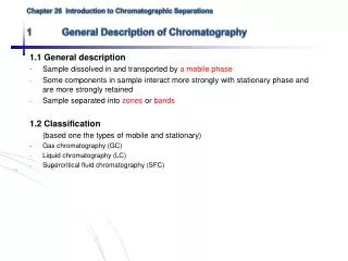
According to the nature of the mobile phase, chromatographic techniques can be classified into three classes: • Liquid chromatography (LC) • Gas chromatography (GC) • Supercritical fluid chromatography (SFC) Other classifications are also available where the term column chromatography where chromatographic separations take place inside a column, and planar chromatography, where the stationary phase is supported on a planar flat plate, are also used.
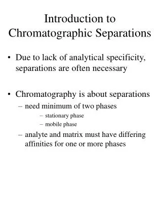
General Description of Chromatography In a chromatographic separation of any type, different components of a sample are transported in a mobile phase (a gas, a liquid, or a supercritical fluid). The mobile phase (also called eluent) penetrates or passes through a solid or immiscible stationary phase. Solutes (eluates) in the sample usually have differential partitioning or interactions with the mobile and stationary phases. Since the stationary phase is the fixed one then those solutes which have stronger interactions with the stationary phase will tend to move slower (have higher retention times) than others which have lower or no interactions with the stationary phase will tend to move faster.
Therefore, chromatographic separations are a consequence of differential migration of solutes. It should be remembered that maximum interactions between a solute and a stationary phase take place when both have similar characteristics, for example in terms of polarity. However, when their properties are so different, a solute will not tend to stay and interact with the stationary phase and will thus prefer to stay in the mobile phase and move faster; a polar solvent and a non polar stationary phase is a good example.
Elution Chromatography The term elution refers to the actual process of separation. A small volume of the sample is first introduced at the top of the chromatographic column. Elution involves passing a mobile phase inside the column whereby solutes are carried down the stream but on a differential scale due to interactions with the stationary phase. As the mobile phase continues to flow, solutes continue to move downward the column. Distances between solute bands become greater with time and as solutes start to leave the column they are sequentially detected.
The time a solute spends in a column (retention time) depends on the fraction of time that solute spends in the mobile phase. As solutes move inside the column, their concentration zone continues to spread and the extent of spreading (band broadening) depends on the time a solute spends in the columns. Factors affecting band broadening are very important and will be discussed later. The dark colors at the center of the solute zones in the above figure represent higher concentrations than are concentrations at the sides. This can be represented schematically as:
Chromatograms The plot of detector signal (absorbance, fluorescence, refractive index, etc..) versus retention time of solutes in a chromatographic column is referred to as a chromatogram. The areas under the peaks in a chromatogram are usually related to solute concentration and are thus very helpful for quantitative analysis. The retention time of a solute is a characteristic property of the solute which reflects its degree of interaction with both stationary and mobile phases. Retention times serve qualitative analysis parameters to identify solutes by comparison with standards.
Migration Rates of Solutes The concepts which will be developed in this section will be based on separation of solutes using a liquid mobile phase and an immiscible liquid stationary phase. This case is particularly important as it is a description of the most popular processes.
Distribution Constants Solutes traveling inside a column will interact with both the stationary and mobile phases. If, as is our case, the two phases are immiscible, partitioning of solutes takes place and a distribution constant, K, can be written: K = CS/CM (1) Where; CS and CM are the concentrations of solute in the stationary and mobile phases, respectively. If a chromatographic separation obeys equation 1, the separation is called linear chromatography. In such separations peaks are Gaussian and independent of the amount of injected sample
The time required for an analyte to travel through the column after injection till the analyte peak reaches the detector is termed the retention time. If the sample contains an unretained species, such species travels with the mobile phase where the time spent by that species to exit the column is called the dead or void time, tM. Solutes will move towards the detector in different speeds, according to each solute’s nature.
Retention Times tM = retention time of mobile phase (dead time) tR = retention time of analyte (solute) tR’= time spent in stationary phase (adjusted retention time) L = length of the column
Velocity = distance/time length of column/ retention times Velocity of solute: Velocity of mobile phase:
average linear velocity of a solute, v, can be written as: v = L/tR (2) Where, L is the column length and tR is the retention time of the solute. The mobile phase linear velocity, u, can be written as: u = L/tM (3) The linear velocity of solutes is a fraction of the linear velocity of the mobile phase. This can be written as: v = u * moles of solute in mp/total moles of solute
This can be further expanded by substitution for the moles of solute in mp, CMVM, and the total number of moles of solute, CMVM + CSVS. v = u * CMVM / (CMVM + CSVS) Dividing both nominator and denominator by CMVM we get v = u * 1/ (1 + CSVS/ CMVM) (4) Now, let us define a new distribution constant, called the capacity or retention factor, k’, as: k’ = CSVS/ CMVM = K VS/VM (5)
Substitution of 1,2 and 5 in equation 4 we get: L/tR = L/tM * {1/(1 + k’)} Rearrangement gives: tR = tM (1+k’) (6) This equation can also be written as: k’ = (tR – tM)/tM
The Selectivity Factor For two solutes to be separated, they should have different migration rates. This is referred to as having different selectivity factors with regard to a specific solute. The selectivity factor, a, can be defined as: a = kB’/kA’ (7) Therefore, a can be defined also as: a = (tR,B – tM)/ (tR,A – tM) (8) For the separation of A and B from their mixture, the selectivity factor must be more than unity.
The Shapes of Chromatographic Peaks Chromatographic peaks will be considered as symmetrical normal error peaks (Gaussian peaks). This assumption is necessary in order to continue developing equations governing chromatographic performance. However, in many cases tailing or fronting peaks are observed.
Gaussian peaks (normal error curves) are easier to deal with since statistical equations for such curves are well established and will be used for derivation of some basic chromatographic relations. It should also be indicated that as solutes move inside a column, their concentration zones are spread more and more where the zone breadth is related to the residence time of a solute in a chromatographic column.
Plate Theory Solutes in a chromatographic separation are partitioned between the stationary and mobile phases. Multiple partitions take place while a solute is moving towards the end of the column. The number of partitions a solute experiences inside a column very much resembles performing multiple extractions. It may be possible to denote each partitioning step as an individual extraction and the column can thus be regarded as a system having a number of segments or plates, where each plate represents a single extraction or partition process.
Therefore, a chromatographic column can be divided to a number of theoretical plates where eventually the efficiency of a separation increases as the number of theoretical plates (N) increases. In other words, efficiency of a chromatographic separation will be increased as the height of the theoretical plate (H) is decreased.
Column Efficiency and the Plate Theory If the column length is referred to as L, the efficiency of that column can be defined as the number of theoretical plates that can fit in that column length. This can be described by the relation: N = L/H
The plate theory successfully accounts for the Gaussian shape of chromatographic peaks but unfortunately fails to account for zone broadening. In addition, the idea that a column is composed of plates is unrealistic as this implies full equilibrium in each plate which is never true. The equilibrium in chromatographic separations is just a dynamic equilibrium as the mobile phase is continuously moving.
Definition of Plate Height From statistics, the breadth of a Gaussian curve is related to the variance s2. Therefore, the plate height can be defined as the variance per unit length of the column: H = s2/L (9) In other words, the plate height can be defined as column length in cm which contains 34% of the solute at the end of the column (as the solute elutes). This can be graphically shown as:
The peak width can also be represented in terms of time, t, where: t = s/v (10) t = s/(L/tR) (11) The width of the peak at the baseline, W, is related to t by the relation: W = 4t where 96% of the solute is contained under the peak. s = L t/tR s = LW/4tR (12)
s2 = L2W2/16tR2 s2 = HL H = LW2/16tR2 N = 16(tR/W)2 (13) Also, from statistics we have: W1/2 = 2.354 t (14) s2 = LH
s = L t/tR s = L (W1/2/2.354)/tR s2 = L2 (W1/2/2.354)2 /tR2 (15) Substitution in equation 9 gives: LH = L2 (W1/2/2.354)2 /tR2 H = L (W1/2/2.354 tR)2 N = L/H N = 5.54 (tR/W1/2)2 (16) Another way to derive the efficiency equation:
From statistics we know that the standard deviation is supposed to be inversely related to the square root of the number separation stages (theoretical plates): s a 1/N1/2 However, we also know that the standard deviation is proportional to retention time: s a tR We can write: s a tR/N1/2 The proportionality constant is practically = 1 Therefore N = (tR/s)2 It is also true that 95.5% of molecules in a peak are contained within + 2s which means that the base of the peak is equal to 4s ; or Wb/4 = s ; Substitution gives: Therefore N = 16(tR/Wb)2
Asymmetric PeaksThe efficiency, N, can be estimated for an asymmetric chromatographic peak using the relation:
N = 41.7 (tR/W0.1)2 / (A/B + 1.25) (17) Draw a horizontal line across the peak at a height equal to 1/10 of the maximum height. Where W0.1 = peak width at 1/10 height = A + B
Rate Theory Band Broadening Apart from specific characteristics of solutes that cause differential migration, average migration rates for molecules of the same solute are not identical. Three main factors contribute to this behavior:
1. Longitudinal Diffusion Molecules tend to diffuse in all directions because these are always present in a concentration zone as compared to the other parts of the column. This contributes to H as follows: HL = K1DM/V Where, DM is the diffusion of solute in the mobile phase. This factor is not very important in liquid chromatography except at low flow rates.
This contributes to H as follows: HL = K1DM/V Where, DM is the diffusion of solute in the mobile phase. This factor is not very important in liquid chromatography except at low flow rates.
2. Resistance to Mass Transfer Mass transfer through mobile and stationary phases contributes to this type of band broadening. a. Stationary Phase Mass Transfer This contribution can be simply attributed to the fact that not all molecules penetrate to the same extent into the stationary phase. Therefore, some molecules of the same solute tend to stay longer in the stationary phase than other molecules
Quantitatively, this behavior can be represented by the equation: Hs = K2 ds2V/Ds Where ds is the thickness of stationary phase and Ds is the diffusion coefficient of solute in the stationary phase.
b. Mobile Phase Mass Transfer Solute molecules which happen to pass through some stagnant mobile phase regions spend longer times before they can leave. Molecules which do not encounter such stagnant mobile phase regions move faster. Other solute molecules which are located close to column tubing surface will also move slower than others located at the center. Some solutes which encounter a channel through the packing material will move much faster than others.
HM = K3dp2V/DM Where dp is the particle size of the packing.
3. Multiple Path Effects Multiple paths which can be followed by different molecules contribute to band broadening. Such effects can be represented by the equation: HE = K4 dp
The overall contributions to band broadening are then, Ht = HL + HS + HM + HE Where; Ht is the overall height equivalent to a theoretical plate resulting from the contributions of the different factors contributing to band broadening. Ht = k4dp + k1DM/V + K2 ds2V/Ds + K3 dp2V/DM Ht = A + B/V + CSV + CMV