Download
1 / 17
170 likes | 188 Vues
Quantitative phase estimation with a bright field microscope . Sri Rama Prasanna Pavani , Ariel Libertun, Sharon King, and Carol Cogswell Micro Optical – Imaging Systems Laboratory, ECE, University of Colorado at Boulder http://moisl.colorado.edu. Frontiers in Optics 9/18/2007. Bright field.

E N D
Quantitative phase estimation with a bright field microscope Sri Rama Prasanna Pavani, Ariel Libertun, Sharon King, and Carol Cogswell Micro Optical – Imaging Systems Laboratory, ECE, University of Colorado at Boulder http://moisl.colorado.edu Pavani et al - Univ. of Colorado, Boulder Frontiers in Optics 9/18/2007
Bright field Phase contrast DIC Digital Holography Phase imaging – What? How? • Transparent (phase) objects modulate only the phase of light • Convert phase modulations into detectable intensity modulations • Quantitative phase for weak phase objects • No phase wrapping • Halo and shading-off • Only for thin objects • Quantitative phase after reconstruction • No phase wrapping • Polarization sensitive • Only for thin objects • Multiple images • Quantitative phase after reconstruction • Thick phase objects • Single image • Vibration sensitive • Phase wrapping • No quantitative phase Pavani et al - Univ. of Colorado, Boulder
Our method • Amplitude mask in the field diaphragm • Pattern is imaged on the sample • Phase object distorts the pattern • Record the distorted pattern • Analytical formula calculates phase Vs 0.2 0.1 (mm) 0.4 0.2 0 0.2 0.4 (mm) (mm) Pavani et al - Univ. of Colorado, Boulder
Our method – 1D • Analytically relate deformation to the optical path length • Consider a 1D phase object p(x) • Ray R from point A, after refraction, appears as if it originated from B • Deformation t(x) is the distance between A and B Normal Tangent n2 p(x) n1 A B t(x) Pavani et al, “Quantitative structured-illumination phase microscopy”, submitted to Applied Optics, June 07 Pavani et al, “Structured-illumination quantitative phase microscopy”, CMB4, COSI 2007 Pavani et al - Univ. of Colorado, Boulder
Our method – 2D 1D deformations After 1D integrations C1 C2 . . CN Quantitative Phase 2D deformation K1 K2 ………… KN Pavani et al, “Quantitative structured-illumination phase microscopy”, submitted to Applied Optics, June 07 Pavani et al - Univ. of Colorado, Boulder
Simulation X 100 18 9 0 5 0 -5 Calculated Phase Quadratic phase 50 25 0 50 25 0 200 100 200 100 After 1D integrations 1D deformations X 100 18 9 0 5 0 -5 0 100 200 0 100 200 Error 8 4 0 -4 -8 (nm) Error Peak error is 5 orders less than peak phase 0 100 200 Pavani et al - Univ. of Colorado, Boulder
Experimental Results Dot shift X,Y Deformations Original pattern 3 0 -3 360 180 0 240 480 Deformed pattern 3 0 -4 360 180 16.54 0 240 480 Quantitative phase 40 30 20 10 0 Profilometer Our method Object: Drop of optical cement 360 180 Pavani et al - Univ. of Colorado, Boulder 480 240 0
Spatial Resolution • Size and the spacing between dots • Dots sampling the object; must obey Nyquist • Resolution enhancement by shifting d s M M shift right shift down shift diagonally + + + = N N = + + + • If dot size = diffraction limited spot size, quantitative phase imaging with the same resolution as a bright field image is possible Pavani et al - Univ. of Colorado, Boulder
Spatial Resolution • Size and the spacing between dots • Dots sampling the object; must obey Nyquist • Resolution enhancement by shifting d s M M shift right shift down shift diagonally + + + = N N = + + + • If dot size = diffraction limited spot size, quantitative phase imaging with the same resolution as a bright field image is possible • Full resolution single image phase imaging with multi-colored dots Pavani et al - Univ. of Colorado, Boulder
t = Dot shift Phase resolution • Smallest detectable change in path length • Minimum deformation w = detector pixel width M = magnification • Trapezoidal numerical integration s x x Example < M = 100x NA = 0.9 w = 7µm s = 1µm n1 = 1.5 n2 = 1 Pavani et al - Univ. of Colorado, Boulder Depth of field = 753nm
Conclusion • Described wide field, full resolution quantitative phase imaging in a bright field microscope • Phase is calculated from deformation using an analytical formula • Conservative calculations with a 100x objective predict a phase resolution of 155nm Pavani et al - Univ. of Colorado, Boulder
Acknowledgements • Prof. Rafael Piestun • Prof. Gregory Beylkin • Vaibhav Khire CDMOptics PhD Fellowship National Science Foundation Grant No. 0455408 Pavani et al - Univ. of Colorado, Boulder
References • J. W. Goodman, Introduction to Fourier Optics, (Roberts & Company, 2005) • M Pluta, Advanced Light Microscopy, vol 2: Specialised Methods, (Elsevier, 1989) • M. R. Arnison, K. G. Larkin, C. J. R. Sheppard, N. I. Smith, C. J. Cogswell, “Linear phase imaging using differential interference contrast microscopy” Journal of Microscopy 214 (1), 7–12 (2004) • C. Preza, "Rotational-diversity phase estimation from differential-interference-contrast microscopy images," J. Opt. Soc. Am. A 17, 415-424 (2000) • Sharon V. King, Ariel R. Libertun, Chrysanthe Preza, and Carol J. Cogswell, “Calibration of a phase-shifting DIC microscope for quantitative phase imaging,” Proc. SPIE 6443, 64430M (2007) • E. Cuche, F. Bevilacqua, and C. Depeursinge, “Digital holography for quantitative phase-contrast imaging,” Opt. Lett. 24, 291-293 (1999) • P. Marquet, B. Rappaz, P. J. Magistretti, E. Cuche, Y. Emery, T. Colomb, and C. Depeursinge, “Digital holographic microscopy: a noninvasive contrast imaging technique allowing quantitative visualization of living cells with subwavelength axial accuracy,” Opt. Lett. 30, 468-470 (2005) • M. Born and E. Wolf, Principles of Optics, ed. 7, (Cambridge University Press, Cambridge, U.K., 1999). • A. C. Kak, M. Slaney, Principles of Computerized Tomographic Imaging, (IEEE Press, New York, NY, 1988) • A. C. Sullivan, Department of Physics, University of Colorado, Campus Box 390, Boulder, CO 80309, USA and R. McLeod are preparing a manuscript to be called “Tomographic reconstruction of weak index structures in volume photopolymers.” • Huang D, Swanson EA, Lin CP, Schuman JS, Stinson WG, Chang W, Hee MR, Flotte T, Gregory K, Puliafito CA, et al., “Optical coherence tomography,” Science1991 Nov 22;254(5035):1178-81. • A. F. Fercher, C. K. Hitzenberger, “Optical coherence tomography,” Chapter 4 in Progress in Optics 44, Elsevier Science B.V. (2002) • A. F. Fercher, W. Drexler, C. K. Hitzenberger and T. Lasser, “Optical coherence tomography - principles and applications,” Rep. Prog. Phys. 66 239–303 (2003) • M. R. Ayres and R. R. McLeod, "Scanning transmission microscopy using a position-sensitive detector," Appl. Opt. 45, 8410-8418 (2006) • Barone-Nugent, E., Barty, A. & Nugent, K. “Quantitative phase-amplitude microscopy I: optical microscopy,” J. Microsc. 206, 194–203 (2002). • J. Hartmann, "Bemerkungen uber den Bau und die Justirung von Spektrographen," Z. Instrumentenkd. 20, 47 (1900). • I. Ghozeil, “Hartmann and other screen tests,” in Optical Shop Testing, D. Malacara, second edition Wiley, New York, 1992, pp. 367–396. • R. V. Shack and B. C. Platt, “Production and use of a lenticular Hartmann screen,” J. Opt. Soc. Am. 61, 656 (1971). • V. Srinivasan, H. C. Liu, and M. Halioua, “Automated phase-measuring profilometry of 3-D diffuse objects,” Appl. Opt. 23, 3105- (1984) • M. G. L. Gustafsson, “Surpassing the lateral resolution limit by a factor of two using structured illumination microscopy,” Journal of Microscopy 198 (2), 82–87 (2000) • M. D. Feit and J. A. , J. Fleck, "Light propagation in graded-index optical fibers (T)," Appl. Opt. 17, 3990- (1978) • Haralick, Robert M., and Linda G. Shapiro. Computer and Robot Vision, Volume I. Addison-Wesley, 1992. pp. 28-48. Pavani et al - Univ. of Colorado, Boulder
Applications and Future work • Industrial inspection, biological imaging • Extracting information from axial deformation • Extending the depth of field of the system • Fabrication of an amplitude mask with higher spatial resolution Pavani et al - Univ. of Colorado, Boulder
Our method – How? 1 Dimensional analysis (from geometry) (Snell’s law, ) (Taylor expansion) C = 2 (C2 – C1) Pavani et al - Univ. of Colorado, Boulder
Our method – How? M 2 Dimensional analysis N and Apply 1D solution along x and y to obtain P2 Pavani et al - Univ. of Colorado, Boulder
Metrology - Cubic phase mask 120 80 40 0 360 180 480 240 0 Deformation Quantitative OPL profile 140 70 0 Cubic phase mask 360 180 480 240 0 Deformation Quantitative OPL profile Pavani et al - Univ. of Colorado, Boulder