Download
1 / 109
1.09k likes | 1.1k Vues
Chapter 3 Image Enhancement. Image Enhancement. The principal objective of enhancement is to process an image so that the result is more suitable than the original image for a specific application The specific application may determine approaches or techniques for image enhancement

E N D
Image Enhancement • The principal objective of enhancement is to process an image so that the result is more suitable than the original image for a specific application • The specific application may determine approaches or techniques for image enhancement • Image enhancement approaches fall into two broad categories • Spatial domain methods • Frequency domain methods
Spatial Domain Methods • Procedures that operate directly on pixels. g(x,y) = T[f(x,y)] where • f(x,y) is the input image • g(x,y) is the processed image • T is an operator on f defined over some neighborhood of (x,y)
Spatial Domain Methods • Neighborhood of a point (x,y) can be defined by using a square/rectangular (common used) or circular subimage area centered at (x,y) • The center of the subimage is moved from pixel to pixel starting at the top of the corner (x,y)
Spatial Domain Methods • The smallest possible neighborhood is of size 1x1 • s=T(r) ;gray-level transformation • s,r : gray level
Image Negatives Image in the range [0, L-1] It is useful in displaying medical images
Log Transformations s = c log(1+r) c : constant, r >= 0 We use a transformation of this type to expand the values of dark pixels while compressing the higher-level values The opposite is true of the inverse log transformation
Power-Law Transformations s = cr • c and are positive constants • Power-law curves with fractional values of map a narrow range of dark input values into a wider range of output values, with the opposite being true for higher values of input levels. • c = = 1 Identity function
Power-Law Transformations Cathode ray tub (CRT) devices have intensity-to-voltage response that is a power function Exp. varies approximately 1.8 to 2.5. 2.5 tends to produce darker images (from the graph)
Advantage: The form of piecewise functions can be arbitrarily complex Disadvantage: Their specification requires considerably more user input Piecewise-Linear Transformation Functions
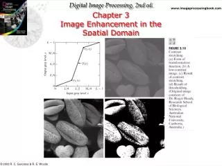
Contrast-stretching • If r1=s1 and r2=s2, linear function produces no changes in gray levels. • If r1=r2, s1=0 and s2=L-1, thresholding • creates a binary image • Intermediate values of (r1, s1)and (r2, s2) • various degrees of spread in the gray levels of the output image, thus affecting its contrast.
Contrast-stretching • increase the dynamic range of the gray levels in the image • (b) a low-contrast image • (c) result of contrast stretching: (r1,s1) = (rmin,0) and (r2,s2) = (rmax,L-1) • (d) result of thresholding
Intensity-Level Slicing • Highlighting a specific range of gray levels in an image • Display a high value of all gray levels in the range of interest and a low value for all other gray levels • (a) transformation highlights range [A,B] of gray level and reduces all others to a constant level • (b) transformation highlights range [A,B] but preserves all other levels
Bit-Plane Slicing Highlighting the contribution made to total image appearance by specific bits
Bit-Plane Slicing Decomposing an image into its planes is useful for analyzing the relative importance of each bit. Determine the number of bits adequate to quantize the image Reconstructing of an image is done by multiplying the pixels in nth plane by the constant 2n-1.
Histogram of a digital image with gray levels in the range [0,L-1] is a discrete function h(rk) = nk Where rk : the kth gray level nk : the number of pixels in the image having gray level rk h(rk) : histogram of a digital image with gray levels rk HistogramProcessing - p(rk) = nk/MN , k=0, 1, …, L-1 - p(rk) is an estimate of the probability of occurrence of gray level k
Histogram Equalization Consider a transformation such as s= T(r), 0 ≤ r ≤ L-1 Assume T(r) satisfies the following conditions (a) T(r) is a monotonically increasing in the interval 0 ≤ r ≤ L-1; (b) 0 ≤ T(r) ≤ 1 for 0 ≤ r ≤ L-1 Monotonically preserves the increasing order from black to white in the image Condition b guarantees that the output gray level will be in the same range as input. Single valued is required to guarantee the inverse transformation will exist r =T-1(s) 0≤ s ≤L-1 To achieve this, T(r) is a strictly monotonically increasing function in the interval 0 ≤r ≤L-1
Histogram Equalization • Let • pr(r) denote the PDF of random variable r • ps (s) denote the PDF of random variable s • If pr(r) and T(r) are known and T-1(s) satisfies condition (a) then ps(s) can be obtained using a formula : • A transformation function is :
The probability of occurrence of gray level in an image is approximated by The discrete version of transformation Histogram Equalization =
Histogram Equalization A 3-bit image 0f size 64×64 pixels (MN =4096) has the intensity distribution shown in the table.
Histogram Matching histogram equalization automatically determines a transformation function that seeks to produce an output image that has a uniform histogram Some applications in which attempting to enhancement based on a uniform histogram is not the best approach The method used to generate a processed image that has a specified histogram is called histogram matching or histogram specification.
Histogram Matching Let r and z denote the gray levels of the input and output (processed) images, respectively. Let s be a random variable with the property We define a random variable z with the property z must satisfy the condition
Histogram Matching • image with a specified probability density function can be obtained from an input image by using the following procedure: • Obtain pr(r) from input image and use the following transformation to get s. 2. Use the specified PDF to obtain the transformation function G(z). 3. Obtain the inverse transformation function The result of this procedure will be an image whose gray levels, z, have the specified probability density function pz(z).
Histogram Matching Find the transformation that will produce an image whose intensity PDF is 1. Find the histogram equalization 2. Find G(z)
Histogram Matching 3. G(z) = s z = G-1(s)
Histogram Matching Discrete Domain Version: Pz(z) is the ith value of the specified histogram For a value of q such that : We find the desired value zq by obtaining the inverse transformation
Histogram Matching • Form the histogram-specified image by • histogram-equalizing the input image • Map every equalized pixel value, sk, of this image to the corresponding value zq in the histogram-specified image. Example: Consider an image 64×64 whose histogram is specified in the figure. It is desired to transform it so that it will have the values specified in the second col. Of the table.
Histogram Matching Obtain the scaled histogram-equalized values (done in the previous example) s0=1, s1=3, s2=5,s3= 6, s4=6, s5=7, s6=7,s7=7.. Compute all the values of the transformation G
Histogram Matching Finally use the mapping from the table to map every pixel in the histogram equalized image into the a corresponding pixel in the newly created histogram-specified image.
Histogram processing methods are global processing, in the sense that pixels are modified by a transformation function based on the gray-level content of an entire image. Sometimes, we may need to enhance details over small areas in an image, which is called a local enhancement. Local Histogram Processing