Download
1 / 63
630 likes | 636 Vues
Chapter 16 Output and the Exchange Rate in the Short Run. Prepared by Iordanis Petsas. To Accompany International Economics: Theory and Policy , Sixth Edition by Paul R. Krugman and Maurice Obstfeld. Chapter Organization. Determinants of Aggregate Demand in an Open Economy

E N D
Chapter 16 Output and the Exchange Rate in the Short Run Prepared by Iordanis Petsas To Accompany International Economics: Theory and Policy, Sixth Edition by Paul R. Krugman and Maurice Obstfeld
Chapter Organization • Determinants of Aggregate Demand in an Open Economy • The Equation of Aggregate Demand • How Output Is Determined in the Short Run • Output Market Equilibrium in the Sort Run: The DD Schedule • Asset Market Equilibrium in the Short Run: The AA Schedule • Short-Run Equilibrium for an Open Economy: Putting the DD and AA Schedules Together
Chapter Organization • Temporary Changes in Monetary and Fiscal Policy • Inflation Bias and Other Problems of Policy Formulation • Permanent Shifts in Monetary and Fiscal Policy • Macroeconomic Policies and the Current Account • Gradual Trade Flow Adjustment and Current Account Dynamics • Summary
Chapter Organization • Appendix I: The IS-LM Model and the DD-AA Model • Appendix II: Intertemporal Trade and Consumption Demand • Appendix III: The Marshall-Lerner Condition and Empirical Estimates of Trade Elasticities
Introduction • Macroeconomic changes that affect exchange rates, interest rates, and price levels may also affect output. • This chapter introduces a new theory of how the output market adjusts to demand changes when product prices are themselves slow to adjust. • A short-run model of the output market in an open economy will be utilized to analyze: • The effects of macroeconomic policy tools on output and the current account • The use of macroeconomic policy tools to maintain full employment
Determinants of Aggregate Demand in an Open Economy • Aggregate demand • The amount of a country’s goods and services demanded by households and firms throughout the world. • The aggregate demand for an open economy’s output consists of four components: • Consumption demand (C) • Investment demand (I) • Government demand (G) • Current account (CA)
Determinants of Aggregate Demand in an Open Economy • Determinants of Consumption Demand • Consumption demand increases as disposable income (i.e., national income less taxes) increases at the aggregate level. • The increase in consumption demand is less than the increase in the disposable income because part of the income increase is saved.
Determinants of Aggregate Demand in an Open Economy • Determinants of the Current Account • The CA balance is viewed as the demand for a country’s exports (EX) less that country's own demand for imports (IM). • The CA balance is determined by two main factors: • The domestic currency’s real exchange rate against foreign currency (q = EP*/P) • Domestic disposable income (Yd)
Determinants of Aggregate Demand in an Open Economy • How Real Exchange Rate Changes Affect the Current Account • An increase in q raises EX and improves the domestic country’s CA. • Each unit of domestic output now purchases fewer units of foreign output, therefore, foreign will demand more exports. • An increase q can raise or lower IM and has an ambiguous effect on CA. • IM denotes the value of imports measured in terms of domestic output.
Determinants of Aggregate Demand in an Open Economy • There are two effects of a real exchange rate: • Volume effect • The effect of consumer spending shifts on export and import quantities • Value effect • It changes the domestic output worth of a given volume of foreign imports. • Whether the CA improves or worsens depends on which effect of a real exchange rate change is dominant. • We assume that the volume effect of a real exchange rate change always outweighs the value effect.
Determinants of Aggregate Demand in an Open Economy • How Disposable Income Changes Affect the Current Account • An increase in disposable income (Yd) worsens the CA. • A rise in Ydcauses domestic consumers to increase their spending on all goods.
Determinants of Aggregate Demand in an Open Economy Table 16-1: Factors Determining the Current Account
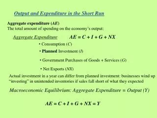
The Equation of Aggregate Demand • The four components of aggregate demand are combined to get the total aggregate demand: D = C(Y – T) + I + G + CA(EP*/P, Y – T) • This equation shows that aggregate demand for home output can be written as: D = D(EP*/P, Y – T, I, G)
The Equation of Aggregate Demand • The Real Exchange Rate and Aggregate Demand • An increase in q raises CA and D. • It makes domestic goods and services cheaper relative to foreign goods and services. • It shifts both domestic and foreign spending from foreign goods to domestic goods. • A real depreciation of the home currency raises aggregate demand for home output. • A real appreciation lowers aggregate demand for home output.
The Equation of Aggregate Demand • Real Income and Aggregate Demand • A rise in domestic real income raises aggregate demand for home output. • A fall in domestic real income lowers aggregate demand for home output.
Aggregate demand, D Aggregate demand function, D(EP*/P, Y – T, I, G) 45° Output (real income), Y The Equation of Aggregate Demand Figure 16-1: Aggregate Demand as a Function of Output
How Output Is Determined in the Short Run • Output market is in equilibrium in the short-run when real output, Y, equals the aggregate demand for domestic output: Y = D(EP*/P, Y – T, I, G) (16-1)
Aggregate demand, D Aggregate demand = aggregate output, D = Y Aggregate demand 3 1 D1 2 45° Y2 Y1 Output, Y Y3 How Output Is Determined in the Short Run Figure 16-2: The Determination of Output in the Short Run
Output Market Equilibrium in the Short Run: The DD Schedule • Output, the Exchange Rate, and Output Market Equilibrium • With fixed price levels at home and abroad, a rise in the nominal exchange rate makes foreign goods and services more expensive relative to domestic goods and services. • Any rise in q will cause an upward shift in the aggregate demand function and an expansion of output. • Any fall in q will cause output to contract.
Aggregate demand, D D = Y Currency depreciates Aggregate demand (E2) 2 Aggregate demand (E1) 1 45° Y1 Output, Y Y2 Output Market Equilibrium in the Short Run: The DD Schedule Figure 16-3: Output Effect of a Currency Depreciation with Fixed Output Prices
Output Market Equilibrium in the Short Run: The DD Schedule • Deriving the DD Schedule • DD schedule • It shows all combinations of output and the exchange rate for which the output market is in short-run equilibrium (aggregate demand = aggregate output). • It slopes upward because a rise in the exchange rate causes output to rise.
Aggregate demand, D D = Y Aggregate demand (E2) Aggregate demand (E1) Y1 Y2 Output, Y Exchange rate, E DD E2 2 E1 1 Output, Y Y1 Y2 Output Market Equilibrium in the Short Run: The DD Schedule Figure 16-4: Deriving the DD Schedule
Output Market Equilibrium in the Short Run: The DD Schedule • Factors that Shift the DD Schedule • Government purchases • Taxes • Investment • Domestic price levels • Foreign price levels • Domestic consumption • Demand shift between foreign and domestic goods • A disturbance that raises (lowers) aggregate demand for domestic output shifts the DD schedule to the right (left).
Aggregate demand, D D = Y Government spending rises D(E0P*/P, Y – T, I, G2) D(E0P*/P, Y – T, I, G1) Y1 Y2 Output, Y Exchange rate, E DD1 DD2 1 2 E0 Output, Y Y1 Y2 Output Market Equilibrium in the Short Run: The DD Schedule Figure 16-5: Government Demand and the Position of the DD Schedule Aggregate demand curves
Asset Market Equilibrium in the Short Run: The AA Schedule • AA Schedule • It shows all combinations of exchange rate and output that are consistent with equilibrium in the domestic money market and the foreign exchange market.
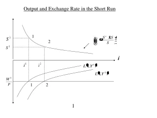
Asset Market Equilibrium in the Short Run: The AA Schedule • Output, the Exchange Rate, and Asset Market Equilibrium • We will combine the interest parity condition with the money market to derive the asset market equilibrium in the short-run. • The interest parity condition describing foreign exchange market equilibrium is: R = R* + (Ee – E)/E where: Ee is the expected future exchange rate R is the interest rate on domestic currency deposits R* is the interest rate on foreign currency deposits
Asset Market Equilibrium in the Short Run: The AA Schedule • The R satisfying the interest parity condition must also equate the real domestic money supply to aggregate real money demand: Ms/P = L(R, Y) • Aggregate real money demand L(R, Y) rises when the interest rate falls because a fall in R makes interest-bearing nonmoney assets less attractive to hold.
Exchange Rate, E Foreign exchange market 2' E2 Domestic interest rate, R 0 R2 MS P Money market Output rises Real money supply 1 Real domestic money holdings Asset Market Equilibrium in the Short Run: The AA Schedule Figure 16-6: Output and the Exchange Rate in Asset Market Equilibrium 1' E1 Domestic-currency return on foreign- currency deposits R1 L(R, Y1) L(R, Y2) 2
Asset Market Equilibrium in the Short Run: The AA Schedule • For asset markets to remain in equilibrium: • A rise in domestic output must be accompanied by an appreciation of the domestic currency. • A fall in domestic output must be accompanied by a depreciation of the domestic currency.
Asset Market Equilibrium in the Short Run: The AA Schedule • Deriving the AA Schedule • It relates exchange rates and output levels that keep the money and foreign exchange markets in equilibrium. • It slopes downward because a rise in output causes a rise in the home interest rate and a domestic currency appreciation.
Exchange Rate, E 1 E1 2 E2 AA Y1 Output, Y Y2 Asset Market Equilibrium in the Short Run: The AA Schedule Figure 16-7: The AA Schedule
Asset Market Equilibrium in the Short Run: The AA Schedule • Factors that Shift the AA Schedule • Domestic money supply • Domestic price level • Expected future exchange rate • Foreign interest rate • Shifts in the aggregate real money demand schedule
Short-Run Equilibrium for an Open Economy: Putting the DD and AA Schedules Together • A short-run equilibrium for the economy as a whole must bring equilibrium simultaneously in the output and asset markets. • That is, it must lie on both DD and AA schedules.
Exchange Rate, E DD 1 E1 AA Y1 Output, Y Short-Run Equilibrium for an Open Economy: Putting the DD and AA Schedules Together Figure 16-8: Short-Run Equilibrium: The Intersection of DD and AA
Exchange Rate, E DD E2 2 E3 3 1 E1 AA Y1 Output, Y Short-Run Equilibrium for an Open Economy: Putting the DD and AA Schedules Together Figure 16-9: How the Economy Reaches Its Short-Run Equilibrium
Temporary Changes in Monetary and Fiscal Policy • Two types of government policy: • Monetary policy • It works through changes in the money supply. • Fiscal policy • It works through changes in government spending or taxes. • Temporary policy shifts are those that the public expects to be reversed in the near future and do not affect the long-run expected exchange rate. • Assume that policy shifts do not influence the foreign interest rate and the foreign price level.
Temporary Changes in Monetary and Fiscal Policy • Monetary Policy • An increase in money supply (i.e., expansionary monetary policy) raises the economy’s output. • The increase in money supply creates an excess supply of money, which lowers the home interest rate. • As a result, the domestic currency must depreciate (i.e., home products become cheaper relative to foreign products) and aggregate demand increases.
Exchange Rate, E DD 2 E2 1 E1 AA2 AA1 Y1 Y2 Output, Y Temporary Changes in Monetary and Fiscal Policy Figure 16-10: Effects of a Temporary Increase in the Money Supply
Temporary Changes in Monetary and Fiscal Policy • Fiscal Policy • An increase in government spending, a cut in taxes, or some combination of the two (i.e, expansionary fiscal policy) raises output. • The increase in output raises the transactions demand for real money holdings, which in turn increases the home interest rate. • As a result, the domestic currency must appreciate.
Exchange Rate, E DD1 DD2 1 E1 2 E2 AA Y1 Output, Y Y2 Temporary Changes in Monetary and Fiscal Policy Figure 16-11: Effects of a Temporary Fiscal Expansion
Temporary Changes in Monetary and Fiscal Policy • Policies to Maintain Full Employment • Temporary disturbances that lead to recession can be offset through expansionary monetary or fiscal policies. • Temporary disturbances that lead to overemployment can be offset through contractionary monetary or fiscal policies.
Exchange Rate, E DD2 DD1 E3 3 2 E2 AA2 1 E1 AA1 Y2 Output, Y Yf Temporary Changes in Monetary and Fiscal Policy Figure 16-12: Maintaining Full Employment After a Temporary Fall in World Demand for Domestic Products
Exchange Rate, E DD1 DD2 E1 1 2 E2 AA1 3 E3 AA2 Y2 Output, Y Yf Temporary Changes in Monetary and Fiscal Policy Figure 16-13: Policies to Maintain Full Employment After a Money-Demand Increase
Inflation Bias and Other Problems of Policy Formulation • Problems of policy formulation: • Inflation bias • High inflation with no average gain in output that results from governments’ policies to prevent recession • Identifying the sources of economic changes • Identifying the durations of economic changes • The impact of fiscal policy on the government budget • Time lags in implementing policies
Permanent Shifts in Monetary and Fiscal Policy • A permanent policy shift affects not only the current value of the government’s policy instrument but also the long-run exchange rate. • This affects expectations about future exchange rates. • A Permanent Increase in the Money Supply • A permanent increase in the money supply causes the expected future exchange rate to rise proportionally. • As a result, the upward shift in the AA schedule is greater than that caused by an equal, but transitory, increase (compare point 2 with point 3 in Figure 16-14).
Exchange Rate, E DD1 2 E2 3 1 E1 AA2 AA1 Yf Y2 Output, Y Permanent Shifts in Monetary and Fiscal Policy Figure 16-14: Short-Run Effects of a Permanent Increase in the Money Supply
Permanent Shifts in Monetary and Fiscal Policy • Adjustment to a Permanent Increase in the Money Supply • The permanent increase in the money supply raises output above its full-employment level. • As a result, the price level increases to bring the economy back to full employment. • Figure 16-15 shows the adjustment back to full employment.
Exchange Rate, E DD2 DD1 2 E2 3 E3 1 AA2 E1 AA3 AA1 Yf Output, Y Y2 Permanent Shifts in Monetary and Fiscal Policy Figure 16-15: Long-Run Adjustment to a Permanent Increase in the Money Supply
Permanent Shifts in Monetary and Fiscal Policy • A Permanent Fiscal Expansion • A permanent fiscal expansion changes the long-run expected exchange rate. • If the economy starts at long-run equilibrium, a permanent change in fiscal policy has no effect on output. • It causes an immediate and permanent exchange rate jump that offsets exactly the fiscal policy’s direct effect on aggregate demand.
Exchange Rate, E DD1 DD2 E1 1 3 AA1 2 E2 AA2 Output, Y Yf Permanent Shifts in Monetary and Fiscal Policy Figure 16-16: Effects of a Permanent Fiscal Expansion Changing the Capital Stock