Independent Samples: Comparing Proportions

1. Independent Samples: Comparing Proportions Lecture 37 Section 11.5 Tue, Nov 6, 2007

2. Comparing Proportions • We wish to compare proportions between two populations. • We should compare proportions for the same attribute in order for it to make sense. • For example, we could measure the proportion of NC residents living below the poverty level and the proportion of VA residents living below the poverty level.

3. Examples • The “gender gap” refers to the difference between the proportion of men who vote Republican and the proportion of women who vote Republican. Men Women

4. Examples • The “gender gap” refers to the difference between the proportion of men who vote Republican and the proportion of women who vote Republican. Dem Dem Rep Rep Men Women

5. Examples • The “gender gap” refers to the difference between the proportion of men who vote Republican and the proportion of women who vote Republican. p1 Dem Dem p2 Rep Rep Men Women p1 > p2

6. Examples • Of course, the “gender gap” could be expressed in terms of the population of Democrats vs. the population of Republicans. Men Men Women Women Democrats Republicans

7. Examples • The proportion of patients who recovered, given treatment A vs. the proportion of patients who recovered, given treatment B. • p1 = recovery rate under treatment A. • p2 = recovery rate under treatment B.

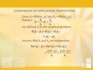
8. Comparing proportions • To estimate the difference between population proportions p1 and p2, we need the sample proportions p1^ and p2^. • The sample difference p1^ – p2^ is an estimator of the true difference p1 – p2.

9. Case Study 13 • City Hall turmoil: Richmond Times-Dispatch poll. • Test the hypothesis that a higher proportion of men than women believe that Mayor Wilder is doing a good or excellent job as mayor of Richmond.

10. Case Study 13 • Let p1 = proportion of men who believe that Mayor Wilder is doing a good or excellent job. • Let p2 = proportion of women who believe that Mayor Wilder is doing a good or excellent job.

11. Case Study 13 • What is the data? • 500 people surveyed. • 48% were male; 52% were female. • 41% of men rated Wilder’s performance good or excellent (p1^ = 0.41). • 37% of men rated Wilder’s performance good or excellent (p2^ = 0.37).

12. Hypothesis Testing • The hypotheses. • H0: p1 – p2 = 0 (i.e., p1 = p2) • H1: p1 – p2 > 0 (i.e., p1 > p2) • The significance level is  = 0.05. • What is the test statistic? • That depends on the sampling distribution of p1^ – p2^.

13. The Sampling Distribution of p1^ – p2^ • If the sample sizes are large enough, then p1^ is N(p1, 1), where and p2^ is N(p2, 2), where

14. The Sampling Distribution of p1^ – p2^ • The sample sizes will be large enough if • n1p1 5, and n1(1 – p1)  5, and • n2p2 5, and n2(1 – p2)  5.

15. Statistical Fact #1 • For any two random variables X and Y,

16. Statistical Fact #2 • Furthermore, if X and Y are both normal, then X – Y is normal. • That is, if X is N(X, X) and Y is N(Y, Y), then

17. The Sampling Distribution of p1^ – p2^ • Therefore, where

18. The Test Statistic • Therefore, the test statistic would be if we knew the values of p1 and p2. • We will approximate them with p1^ and p2^.