Download

1 / 19
190 likes | 359 Vues
A SYSTEMIC RADIOMETRIC CALIBRATION APPROACH FOR LDCM AND THE LANDSAT ARCHIVE – An Update. LDCM Science Team Meeting June 12-14, 2007 Oregon State University. Dennis Helder, EE & CS Dept, SDSU Dave Aaron, Physics Dept, SDSU Jim Dewald, SDSU IP Lab Tim Ruggles, SDSU IP Lab

E N D
A SYSTEMIC RADIOMETRIC CALIBRATION APPROACH FOR LDCM AND THE LANDSAT ARCHIVE – An Update LDCM Science Team Meeting June 12-14, 2007 Oregon State University Dennis Helder, EE & CS Dept, SDSU Dave Aaron, Physics Dept, SDSU Jim Dewald, SDSU IP Lab Tim Ruggles, SDSU IP Lab Chunsun Zhang, SDSU GISc Center
A SYSTEMIC RADIOMETRIC CALIBRATION APPROACH FOR LDCM AND THE LANDSAT ARCHIVE • Consistent calibration of the Landsat archive through use of pseudo-invariant sites • Techniques for relative gain calibration/correction of large linear arrays • Vicarious calibration of LDCM and Landsat TM/ETM+ instruments
Techniques for relative gain calibration/correction of large linear arrays • Relative Gain—whiskbroom to pushbroom scanner issue: • Landsat 4/5 TM—16 detectors/refl. band + 4 thermal det. 100 det. • Landsat 7 ETM+ -- add the pan band & 30m thermal band 136 detectors • Advanced Land Imager 320 multispectral detectors/sca x 4 sca’s/band x 9 bands + 960 pan detectors/sca x 4sca’s/band = 15,360 detectors • LDCM ≥ 57,000 detectors! Relative gain estimation is a critical element for LDCM! • Methods to estimate Relative Gain • Image uniform fields • Statistical based methods • Lifetime data sets • Individual scenes • 90o yaw maneuvers
Relative Gain Estimation Techniques • Lifetime Histogram Statistics Method • Over ‘long’ periods of time each detector observes the same data statistically. • Ratios of detector means or standard deviations can be used to estimate relative gains. • Individual Scene Statistics Method • Odd/Even detector striping most prevalent due to focal plane design • Develop an objective function measuring odd/even striping • Use least squares approach to minimize objective function through estimation optimal relative gains. • Yaw Data Sets • ‘Perfect’ 90o yaw maneuver allows each detector to observe same point on the earth’s surface. Deterministic estimate of relative gain is possible. • Near 90o yaw maneuver provides very uniform scene for relative gain estimate, but not perfect. • Use these data sets with statistical algorithms to develop a more accurate estimate of relative gains.
Scene: EO12001059230136_PF1_01 (Antarctica) Band: 1p SCA: 1
Remove Bias Band 1p
Correction Factors Using Image Statistics Band 1p Correction Factors (1/Relative Gains) Detector Number
Corrected Image Band 1p Data Range 263-384 Data Range 283-386 1st 320 Lines
EO12004262105030_HGS – A YAW IMAGE SCA 1 Band 1p An example of a yaw image… Yaw angle = 88.3o
Band 1p Cont. Data Range: 263-384 Data Range: 278-381 Even and Odd Detectors normalized by equalizing total means.
EO12002329141606_SGS SCA 1 Band 1p A 2nd example of a yaw image… Yaw angle = 88.5o
EO12002329141606_SGS Rel Gains Applied toEO12001059230136_PF1 SCA 1 Band 1p
Band 1p Cont. Data Range: 263-384 Data Range: 279-382 Even and Odd Detectors normalized by equalizing total means.
Band 1p SCA 1 EO12004262105030_HGS (upper images corrected by 2004 yaw scene-based gains) Data Range: 278-381 Data Range: 283-374 EO12001059230136_PF1 (Antarctica) EO12004166105103_HGS (Africa) EO12002329141606_SGS (lower images corrected by 2002 yaw scene-based gains Data Range: 279-382 Data Range: 283-373
EO12001227182254_AGS_01SCA 1 MS-1p Yaw Image-based Correction Lifetime Histogram Statistics Correction
Summary Points • Lifetime statistics provide good information of overall relative gain trends within an array • Assumes relative gains only vary slowly with time • May require ‘fine tuning’ to optimize estimates • Individual scene statistics approach is optimal with regard to visual removal of striping • Addresses problem of small, short term relative gain drift • Needs to be adapted to longer duration data sets • May be excellent for use with yaw images • Use of imagery collected during 90o yaw maneuvers can provide excellent information on detector gains • Need to image uniform surfaces • Should be executed on a regular (monthly to quarterly?) basis • Can be done with minimal impact to normal imaging by considering polar regions and possibly deserts.