Download
1 / 136
1.41k likes | 1.72k Vues
8. Functions of Several Variables Partial Derivatives Maxima and Minima of Functions of Several Variables The Method of Least Squares Constrained Maxima and Minima and the Method of Lagrange Multipliers Double Integrals. Calculus of Several Variables. 8.1. Functions of Several Variables.

E N D
8 • Functions of Several Variables • Partial Derivatives • Maxima and Minima of Functions of Several Variables • The Method of Least Squares • Constrained Maxima and Minima and the Method of Lagrange Multipliers • Double Integrals Calculus of Several Variables
8.1 Functions of Several Variables
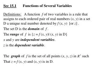
Functions of Two Variables A real-valued function of two variablesf, consists of • A set A of ordered pairs of real numbers (x, y) called the domain of the function. • A rule that associates with each ordered pair in the domain of fone and onlyone real number, denoted by z =f(x, y).
Examples • Let f be the function defined by • Compute f(0, 0), f(1, 2), and f(2, 1). Solution • The domain of a function of two variablesf(x, y), is a set of ordered pairs of real numbers and may therefore be viewed as a subset of thexy-plane. Example 1, page 536
Examples • Find the domain of the function Solution • f(x, y) is defined for all real values of x and y, so the domain of the function f is the set of all points(x, y)in thexy-plane. Example 2, page 536
Examples • Find the domain of the function Solution • g(x, y) is defined for all x≠y, so the domain of the function g is the set of all points(x, y)in thexy-plane exceptthose lying on the y = x line. y y = x x Example 2, page 536
Examples • Find the domain of the function Solution • We require that 1 – x2 – y2 0 or x2 + y2 1 which is the set of all points(x, y) lying on and inside thecircle of radius1 with center at the origin: y 1 –1 x2 + y2= 1 x –1 1 Example 2, page 536
Applied Example: Revenue Functions • Acrosonic manufactures a bookshelf loudspeaker system that may be bought fully assembled or in a kit. • The demand equations that relate the unit price, p and q, to the quantities demanded weekly, x and y, of the assembled and kit versions of the loudspeaker systems are given by • What is the weekly total revenue function R(x, y)? • What is the domain of the function R? Applied Example 3, page 537
Applied Example: Revenue Functions Solution • The weekly revenue from selling x units assembled speaker systems at p dollars per unit isgiven byxp dollars. Similarly, the weekly revenue from selling yspeaker kits at q dollars per unit isgiven byyq dollars. Therefore, the weekly total revenuefunctionR is given by Applied Example 3, page 537
Applied Example: Revenue Functions Solution • To find the domain of the functionR, note that the quantities x, y, p, and q must be nonnegative, which leads to the following system of linear inequalities: Thus, the graph of the domain is: y 2000 1000 D x 1000 2000 Applied Example 3, page 537
Graphs of Functions of Two Variables • Consider the task of locating P(1, 2, 3) in 3-space: • One method to achieve this is to start at theoriginand measure out from there, axis by axis: z P(1, 2, 3) 3 y 1 2 x
Graphs of Functions of Two Variables • Consider the task of locating P(1, 2, 3) in 3-space: • Another common method is to find thexycoordinate and from there elevate to the level of the z value: z P(1, 2, 3) 3 y 2 1 (1, 2) x
Graphs of Functions of Two Variables • Locate the following points in 3-space: Q(–1, 2, 3),R(1, 2, –2),andS(1, –1, 0). Solution z Q(–1, 2, 3) 3 y S(1, –1, 0) –2 x R(1, 2, –2)
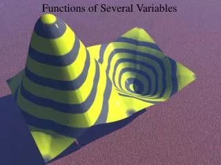
Graphs of Functions of Two Variables • The graph of a function in 3-space is a surface. • For every (x, y) in the domain of f, there is a z value on the surface. z z = f(x, y) (x, y, z) y (x, y) x
Level Curves • The graph of a function of two variables is often difficult to sketch. • It can therefore be useful to apply the method used to construct topographic maps. • This method is relatively easy to apply and conveys sufficient information to enable one to obtain a feel for the graph of the function.
Level Curves • In the 3-space graph we just saw, we can delineate the contour of the graph as it is cut by a z = c plane: z z = f(x, y) z = c y f(x, y) = c x
Examples • Sketch a contour map of the function f(x, y) = x2 + y2. Solution • The function f(x, y) = x2 + y2 is a revolving parabola called a paraboloid. z f(x, y) = x2 + y2 y Example 5, page 540 x
Examples • Sketch a contour map of the function f(x, y) = x2 + y2. Solution • A level curve is the graph of the equation x2 + y2 = c, which describes a circle with radius . • Taking different values of c we obtain: z f(x, y) = x2 + y2 y x2 + y2 = 16 4 2 –2 –4 x2 + y2 = 9 x2 + y2 = 4 x2 + y2 = 1 x2 + y2 = 16 x2 + y2 = 0 x –4 –2 2 4 x2 + y2 = 9 x2 + y2 = 4 x2 + y2 = 1 y x2 + y2 = 0 Example 5, page 540 x
Examples • Sketch level curves of the function f(x, y) = 2x2 – y corresponding to z = –2, –1, 0, 1, and 2. Solution • The level curves are the graphs of the equation 2x2 – y= k or for k = –2, –1, 0, 1, and 2: y 2x2 – y= –2 4 3 2 1 0 –1 –2 2x2 – y= –1 2x2 – y= 0 2x2 – y= 1 2x2 – y= 2 x –2 –1 1 2 Example 6, page 540
8.2 Partial Derivatives
First Partial Derivatives First Partial Derivatives of f(x, y) • Suppose f(x, y) is a function of two variablesx and y. • Then, the first partial derivative of fwith respect to xatthe point(x, y) is provided the limit exists. • The first partial derivative of fwith respect to yatthe point(x, y) is provided the limit exists.
Geometric Interpretation of the Partial Derivative z f(x, y) y x
Geometric Interpretation of the Partial Derivative z f(x, y) f(x, b) y = bplane b y a (a, b) x
Geometric Interpretation of the Partial Derivative z f(x, y) y x
Geometric Interpretation of the Partial Derivative z f(x, y) f(c, y) x = c plane d y c (c, d) x
Examples • Find the partial derivatives∂f/∂xand ∂f/∂yof the function • Use the partials to determine the rate of change of f in the x-direction and in the y-direction at the point (1, 2) . Solution • To compute ∂f/∂x, think of the variabley as a constant and differentiate the resulting function of xwith respect tox: Example 1, page 546
Examples • Find the partial derivatives∂f/∂xand ∂f/∂yof the function • Use the partials to determine the rate of change of f in the x-direction and in the y-direction at the point (1, 2). Solution • To compute ∂f/∂y, think of the variablex as a constant and differentiate the resulting function of ywith respect toy: Example 1, page 546
Examples • Find the partial derivatives∂f/∂xand ∂f/∂yof the function • Use the partials to determine the rate of change of f in the x-direction and in the y-direction at the point (1, 2). Solution • The rate of change of f in the x-direction at the point (1, 2) is given by • The rate of change of f in the y-direction at the point (1, 2) is given by Example 1, page 546
Examples • Find the firstpartial derivativesof the function Solution • To compute ∂w/∂x, think of the variabley as a constant and differentiate the resulting function of xwith respect tox: Example 2, page 547
Examples • Find the firstpartial derivativesof the function Solution • To compute ∂w/∂y, think of the variablex as a constant and differentiate the resulting function of ywith respect toy: Example 2, page 547
Examples • Find the firstpartial derivativesof the function Solution • To compute ∂g/∂s, think of the variablet as a constant and differentiate the resulting function of swith respect tos: Example 2, page 547
Examples • Find the firstpartial derivativesof the function Solution • To compute ∂g/∂t, think of the variables as a constant and differentiate the resulting function of twith respect tot: Example 2, page 547
Examples • Find the firstpartial derivativesof the function Solution • To compute ∂h/∂u, think of the variablev as a constant and differentiate the resulting function of uwith respect tou: Example 2, page 547
Examples • Find the firstpartial derivativesof the function Solution • To compute ∂h/∂v, think of the variableu as a constant and differentiate the resulting function of vwith respect tov: Example 2, page 547
Examples • Find the firstpartial derivativesof the function Solution • Here we have a function ofthree variables, x,y, and z, and we are required to compute • For short, we can label these first partial derivatives respectively fx, fy, and fz. Example 3, page 549
Examples • Find the firstpartial derivativesof the function Solution • To find fx, think of the variablesy and z as a constant and differentiate the resulting function of xwith respect tox: Example 3, page 549
Examples • Find the firstpartial derivativesof the function Solution • To find fy, think of the variablesx and z as a constant and differentiate the resulting function of ywith respect toy: Example 3, page 549
Examples • Find the firstpartial derivativesof the function Solution • To find fz, think of the variablesx and y as a constant and differentiate the resulting function of zwith respect toz: Example 3, page 549
The Cobb-Douglas Production Function • The Cobb-Douglass Production Function is of the form f(x, y) = axby1–b (0 < b < 1) where a and b are positive constants, x stands for the cost of labor, y stands for the cost of capital equipment, and f measures the output of the finished product.
The Cobb-Douglas Production Function • The Cobb-Douglass Production Function is of the form f(x, y) = axby1–b (0 < b < 1) • The first partial derivativefxis called the marginal productivity of labor. • It measures the rate of change of production with respect to the amount of money spent on labor, with the level of capital kept constant. • The first partial derivativefyis called the marginal productivity of capital. • It measures the rate of change of production with respect to the amount of money spent on capital, with the level of labor kept constant.
Applied Example: Marginal Productivity • A certain country’s production in the early years following World War II is described by the function f(x, y) =30x2/3y1/3 when x units of labor and y units of capital were used. • Compute fx and fy. • Find the marginal productivity of labor and the marginal productivity of capital when the amount expended on labor and capital was 125 units and 27 units, respectively. • Should the government have encouraged capital investment rather than increase expenditure on labor to increase the country’s productivity? Applied Example 4, page 550
Applied Example: Marginal Productivity f(x, y) =30x2/3y1/3 Solution • The first partial derivatives are Applied Example 4, page 550
Applied Example: Marginal Productivity f(x, y) =30x2/3y1/3 Solution • The required marginal productivity of labor is given by or 12 units of output per unit increase inlabor expenditure (keeping capital constant). • The required marginal productivity of capital is given by or 27 7/9 units of output per unit increase incapital expenditure (keeping labor constant). Applied Example 4, page 550
Applied Example: Marginal Productivity f(x, y) =30x2/3y1/3 Solution • The government should definitely have encouraged capital investment. • A unitincrease in capital expenditure resulted in a much faster increase in productivity than a unitincrease in labor: 27 7/9 versus 12 per unit of investment, respectively. Applied Example 4, page 550
Second Order Partial Derivatives • The first partial derivativesfx(x, y) andfy(x, y) of a function f(x, y) of two variables x and y are also functions of x and y. • As such, we may differentiate each of the functions fx and fy to obtain the second-order partial derivatives of f.
Second Order Partial Derivatives • Differentiating the function fxwith respect tox leads to the second partial derivative • But the function fx can also be differentiatedwith respect toy leading to a different second partial derivative
Second Order Partial Derivatives • Similarly, differentiating the function fywith respect toy leads to the second partial derivative • Finally, the function fy can also be differentiatedwith respect tox leading to the second partial derivative
Second Order Partial Derivatives • Thus, foursecond-order partial derivatives can be obtained of a function of two variables: When both are continuous
Examples • Find the second-order partial derivatives of the function Solution • First, calculate fx and use it to find fxx and fxy: Example 6, page 552
Examples • Find the second-order partial derivatives of the function Solution • Then, calculate fy and use it to find fyx and fyy: Example 6, page 552