Download
1 / 1
10 likes | 140 Vues
LFM. J ll , n p ,T p. E. Magnetosphere - Ionosphere Coupler. ( H + P ) = J ll -J w. Particle precipitation: F e , E 0. Conductivities: p , h, Winds: J w. Electric Potential: tot. TIE-GCM. GSWM. Response of the Ionosphere to the December 2006 Storm: CMIT Simulation

E N D
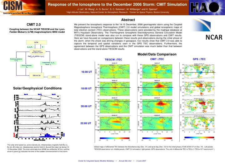
LFM Jll, np,Tp E Magnetosphere - Ionosphere Coupler (H+P)=Jll-Jw Particle precipitation: Fe, E0 Conductivities: p, h, Winds: Jw Electric Potential: tot TIE-GCM GSWM Response of the Ionosphere to the December 2006 Storm: CMIT Simulation J. Lei1, W. Wang1, A. G. Burns1, S. C. Solomon1, M. Wiltberger1 and H. Spence2 1High Altitude Observatory, National Center for Atmospheric Research; 2Center for Space Physics, Boston University Abstract We present the ionospheric response to the 14-15 December, 2006 geomagnetic storm using the Coupled Magnetosphere Ionosphere Thermosphere (CMIT) 2.0 model simulations and global ionospheric maps of total electron content (TEC) observations. These observations were provided by the madrigal database at MIT’s Haystack Observatory. The Thermosphere Ionosphere Electrodynamics General Circulation Model (TIEGCM) stand-alone model was also run to compare with these GPS observations and CMIT results. Here we have focused on comparisons between these results and observations during the initial phase of the storm, when the shock was driving changes in geospace. Our results show that CMIT 2.0 was able to capture the temporal and spatial variations seen in the GPS TEC observations. Furthermore, the agreement between the GPS observations and the CMIT simulation was much better than that between observations and the stand-alone TIEGCM results. CMIT 2.0 Coupling between the NCAR TIEGCM and the Lyon-Fedder-Mobarry (LFM) magnetospheric MHD model Model/Data Comparison CMIT ∆TEC GPS ∆TEC TIEGCM ∆TEC 16:00 UT Solar/Geophysical Conditions 18:00 UT 20:00 UT 22:00 UT The solar wind speed (a), proton density (b), interplanetary magnetic field By (c), Bz (d), AE index (e), interplanetary electric field (f), Ap and Dst index (g) during 13-15 December 2006.The solar wind data from WIND are shifted by 30 min, and the arrow in panel (g) indicates the time of the sudden commencement of this storm. Global maps of differential TEC between the disturbance day (Dec. 14 ) and quiet day (Dec. 13) for the initial phase (14:00-23:00 UT on Dec. 14). Left panels: TIEGCM stand-alone run; middle panels: CMIT 2.0 simulation; right panels: GPS observations. The unit of differential TEC is TECu (1 TECu=1016 electrons/m2). Center for Integrated Space Weather Modeling • Annual Site Visit • 5 June 2007