Download
1 / 23
240 likes | 678 Vues
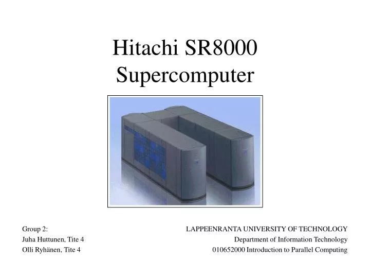
Hitachi SR8000 Supercomputer. LAPPEENRANTA UNIVERSITY OF TECHNOLOGY Department of Information Technology 010652000 Introduction to Parallel Computing. Group 2: Juha Huttunen, Tite 4 Olli Ryhänen, Tite 4. History of SR8000.

E N D
Hitachi SR8000Supercomputer LAPPEENRANTA UNIVERSITY OF TECHNOLOGY Department of Information Technology 010652000 Introduction to Parallel Computing Group 2: Juha Huttunen, Tite 4 Olli Ryhänen, Tite 4
History of SR8000 • Successor of Hitachi S-3800 vector super computer and SR2201 parallel computer.
Overview of system architecture • Distributed-memory parallel computer with pseudo-vector SMP nodes.
Processing Unit • IBM PowerPC CPU architecture with Hitachi’s extensions • 64 bit PowerPC RISC processors • Available in speeds: 250MHz, 300MHz, 375MHz and 450MHz • Hitachi extensions • Additional 128 floating-point registers (total of 160 FPRs) • Fast hardware barrier synchronisation mechanism • Pseudo Vector Processing (PVP)
160 Floating-Point registers • 160 FP registers • FR0 – FR31 global part • FR32 – FR128 slide part • FPR operations extended to handle slide part Inner Product of two arrays
Pseudo Vector Processing (PVP) • Introduced in Hitachi SR2201 supercomputer • Designed to solve memory bandwidth problems in RISC CPUs • Performance similar of vector processor • Non-blocking arithmetic execution • Reduce chances of cache misses • Pipelined data loading • pre-fetch • pre-load
Pseudo Vector Processing (PVP) • Performance effect of PVP
Node Structure • Pseudo vector SMP-nodes • 8 instruction processors (IP) for computation • 1 system control processor (SP) for management • Co-operative Micro-processors in single Address Space (COMPAS) • Maximum number of nodes is 512 (4096 processors) • Node types • Processing Nodes (PRN) • I/O Nodes (ION) • Supervisory Node (SVN) • One per system
Node Partitioning/Grouping • A physical node can belong to many logical partitions • A node can belong to multiple node groups • Node groups are created dynamically by the master node
COMPAS • Auto parallelization by the compiler • Hardware support for fast fork/join sequences • Small start-up overhead • Cache coherency • Fast signalling between child and parent processes
COMPAS • Performance effect of COMPAS
Interconnection Network • Interconnection network • Multidimensional crossbar • 1, 2 or 3-dimensional • Maximum of 8 nodes/dimension • External connections via I/O nodes • Ethernet, ATM, etc. • Remote Direct Memory Access (RDMA) • Data transfer between nodes • Minimizes operating system overhead • Support in MPI and PVM libraries
Software on SR8000 • Operating System • HI-UX with MPP (Massively Parallel Processing) features • Built-in maintenance tools • 64 bit addressing with 32 bit code support • Single system for the whole computer • Programming tools • Optimized F77, F90, Parallel Fortran, C and C++ compilers • MPI-2 (Message Parsing Interface) • PVM (Parallel Virtual Machine) • Variety of debugging tools (eg. Vampir and Totalview)
Hybrid Programming Model • Supports several parallel programming methods • MPI + COMPAS • Each node has one MPI process • Pseudo vectorization by PVP • Auto parallelization by COMPAS • MPI + OpenMP • Each node has one MPI process • Divided to threads between the 8 CPUs by OpenMP • MPI + MPP • Each CPU has one MPI process (max 8 processes/node) • COMPAS • Each node has one process • Pseudo vectorization by PVP • Auto parallelization by COMPAS
Hybrid Programming Model • OpenMP • Each node has one process • Divided to threads between the 8 CPUs by OpenMP • Scalar • One application with a single thread on one CPU • Can use the 9th CPU • ION • Default model for commands like ’ls’, ’vi’ etc. • Can use the 9th CPU
Hybrid Programming ModelPerformance Effects • Parallel vector-matrix multiplication used as example
Performance Figures • 10 places on the Top 500 list • Highest rankings 26 and 27 • Theoretical maximum performance 7,3Tflop/s with 512 nodes • Node performance depends on the model, from 8Gflop/s to 14,4Gflop/s depending on the CPU speed. • Maximum memory capacity 8TB • Latency from processor to various locations • To memory: 30 – 200 nanoseconds • To remote memory via RDMA feature: ~3-5 microseconds • MPI (without RDMA): ~6-20 microseconds • To disk: ~8 milliseconds • To tape: ~30 seconds
Scalability • Highly scalable architecture • Fast interconnection network and modular node structure • Externally coupling 2 G1 frames performance of 1709Gflop/s out of 2074Gflop/s was achieved (82% efficiency)
Leibniz-Rechenzentrum • SR8000-F1 in Leibniz-Rechenzentrum (LRZ), Munich • German federal top-level compute server in Bavaria • System information • 168 nodes (1344 processors, 375 MHz) • 1344GB of memory • 8 GB/node • 4 nodes with 16 GB • 10TB of disk storage
Leibniz-Rechenzentrum • Performance • Peak performance per CPU – 1,5 GFlop/s (per node 12 GFlop/s) • Total peak performance – 2016 GFlop/s (Linpack 1645 GFlop/s) • I/O bandwidth – to /home 600 MB/s, to /tmp 2,4GB/s • Expected efficiency (from LRZ benchmarks) • >600 GFlop/s • Performance from main memory (most unfavourable case) • >244 GFlop/s
Leibniz-Rechenzentrum • Unidirectional communication bandwidth: • MPI without RDMA – 770 MB/s • MPI without RDMA – 950 MB/s • Hardware – 1000 MB/s • 2*unidirectional bisection bandwidth • MPI and RDMA – 2x79 = 158 GB/s • Hardware – 2x84 = 168 GB/s