Download
1 / 40
400 likes | 523 Vues
Atmospheric Correction for Turbid Waters in Coastal Regions: Need Bands > 1000 nm. Menghua Wang NOAA/NESDIS/ORA E/RA3, Room 102, 5200 Auth Rd. Camp Springs, MD 20746, USA Menghua.Wang@noaa.gov The Coastal Ocean Applications and Science Team Meeting

E N D
Atmospheric Correction for Turbid Waters in Coastal Regions: Need Bands > 1000 nm Menghua Wang NOAA/NESDIS/ORA E/RA3, Room 102, 5200 Auth Rd. Camp Springs, MD 20746, USA Menghua.Wang@noaa.gov The Coastal Ocean Applications and Science Team Meeting September 7-8, 2005, Corvallis, Oregon
Solar Irradiance Passive Remote Sensing: Sensor-measured signals are all originated from the sun!
Ocean Color Remote Sensing Sensor-Measured “Green” ocean Blue ocean Atmospheric Correction (removing >90% signals) Calibration (0.5% error in TOA >>>> 5% in surface) From H. Gordon
Atmospheric Windows UV bandscan be used for detecting the absorbing aerosol cases Two long NIR bands (1000 & 1240 nm)are useful for of the Case-2 waters
The Ocean Radiance Spectrum TOA Reflectance Open Ocean Waters Coastal Waters
Atmospheric Correction MODISand SeaWiFS algorithm (Gordon and Wang 1994) • wis thedesired quantity in ocean color remote sensing. • Tgis the sun glint contribution—avoided/masked/corrected. • Twcis the whitecap reflectance—computed from wind speed. • risthe scattering from molecules—computed using the Rayleigh lookup tables (atmospheric pressure dependence). • A = a+rais the aerosol and Rayleigh-aerosol contributions —estimated using aerosol models. • For Case-1 waters at the open ocean,wis usually negligibleat750 & 865 nm. A can be estimated using these two NIR bands. Ocean is usually not black at NIR for the coastal regions. Gordon, H. R. and M. Wang, “Retrieval of water-leaving radiance and aerosol optical thickness over the oceans with SeaWiFS: A preliminary algorithm,” Appl. Opt., 33, 443-452, 1994.
SeaWiFS Chlorophyll-a Concentration(October 1997-December 2003)
SeaWiFS experiences demonstrate that the atmospheric correction works well in the open oceans.
SeaWiFSGlobal Deep Ocean Results Wang, M., K. Knobelspiesse, and C. R. McClain, “Study of the SeaWiFS aerosol optical property data over ocean in combination with the ocean color products,” J. Geophys. Res., 110, D10S06, doi:10.1029/2004JD004950.
Turbid Waters: Examples from MODIS Data (Short Wave Infrared Bands for Coastal Regions) Wang, M. and W. Shi, “Estimation of ocean contribution at the MODIS near-infrared wavelengths along the east coast of the U.S.: Two case studies,” Geophys. Res. Letters,32, L13606, doi:10.1029/2005GL022917 (2005).
Case-2 Water Complications For productive ocean waters at coastal regions, the ocean is usually not black at the NIR wavelengths at 765 and 865 nm. In these cases, the ocean contributions at the NIR are often mistakenly accounted as radiance scattering from atmosphere, thereby leading to over-correction of atmospheric radiance and underestimation of water-leaving radiance at the visible. Examples of atmospheric correction for the non-black ocean at the NIR bands. Negative nLw
Atmospheric Correction:Short Wave Infrared (SWIR) • In general, to effect the atmospheric correction operationally using the NIR bands at 765 and 865 nm, or using the spectral optimization with measurements from 412-865nm, Case-2 bio-optical model that has strongly regional & temporal dependences is needed. • At the short wave infrared (SWIR) wavelengths (>~1000 nm), ocean water is much strongly absorbing and ocean contributions are significant less. Thus, atmospheric correction may be carried out at the coastal regions without using the bio-optical model. • Examples using the MODIS 1240 and 1640 nm data to derive the ocean contributions at the NIR bands. • We use the SWIR (1640 nm) for the cloud masking. This is necessary for the coastal region waters.
Water Absorption Relative to 865 nm Black Ocean at the SWIR bands:Absorption at the SWIR bands is an order larger than that at the 865 nm
The Rayleigh-Corrected TOA Reflectance Identified as clouds using 869 nm Cloud Masking:Need bands > ~ 1000 nm
The Rayleigh-Corrected TOA Reflectance Identified as clouds using 869 nm Cloud Masking:Need bands > ~ 1000 nm
The Rayleigh-Corrected TOA Reflectance Identified as clouds using 869 nm Cloud Masking:Need bands > ~ 1000 nm
Aerosol Single-Scattering Epsilon (0 = 1640nm) Spectral aerosol contribution relative to wavelength 1640 nm for 12 models
Data Processing Using SWIR Bands Lookup Tables Generation and Implementation: • Rayleigh lookup tables for the SWIR bands. • Aerosol optical property data (scattering phase function, single scattering albedo, extinction coefficients) for the SWIR bands (12 models same as for SeaWiFS/MODIS). • Aerosol lookup tables (12 aerosol models--same as for SeaWiFS/MODIS) for the SWIR bands. Data Processing: • Developed cloud masking using the 1640 nm band. This is necessary for the high-productive waters (e.g., coastal regions). • Implemented the sun glint mask.
MODIS-Measured TOAvs. TheoreticalTOA Open Ocean, MODIS Terra Granule 20041071625 Need vicarious calibration for 1240 and 1640 nm bands:Adjusting the gains so that the intercept=0 and slope=1.
MODIS Terra L1b Vicarious Calibration B1240 and B1640 at open ocean Aerosol Type from B1240 and B1640 Reflectance w/o Ocean Contribution (B748, B865) Ocean-Contributed Reflectance (B748, B865) Procedures For the MODIS 748 and 869 nm Bands Ocean-Contributed Reflectance Estimation
Histogram of Ocean Contributed Reflectance (Open Ocean)
MODIS Terra Granule:20040711515 (March 11, 2004) The Rayleigh-Corrected TOA Reflectance 748 nm 869 nm 1240 nm 1640 nm Rayleigh-Removed
The NIR Ocean Contributions Very large ocean contribution at the NIR bands in coastal regions with significant spatial & temporal variations.
Real values VS Theoretical Values (20040711825) MODIS Aqua 2130 nm MODIS Aqua 1240 nm
Band 748 Band 869 Ocean-Contributed Reflectance (AQUA 20040711825) B1240-2130 Atmospheric Correction B1240-2130 Atmospheric Correction
Ocean-Contributed Reflectance at NIR Very significant ocean contributions!
Conclusions • Both SeaWiFS/MODIS provide high quality ocean color products in the open oceans. • For the turbid waters in coastal regions, ocean is not black at the NIR bands. This leads to underestimation of the sensor-measured water-leaving radiances with current SeaWiFS/MODIS atmospheric correction algorithm. • Ocean is black for turbid waters at wavelengths >~1000 nm. Thus, the longer NIR bands can be used for atmospheric correction over the turbid waters. • In addition, we need longer NIR bands for cloud masking in the coastal regions. • We need longer NIR bands (> ~1000 nm) for GOES-R HES-CW for atmospheric correction for turbid waters in coastal regions.