Download
1 / 18
190 likes | 191 Vues
This study aims to improve global wind-wave probabilistic forecasts and products beyond week 2 by applying MLP neural networks to nonlinear ensemble averaging. The study includes tests at single locations, neural network architectures, spatial distribution of wind and wave climates, and evaluation using NDBC buoys and altimeters.

E N D
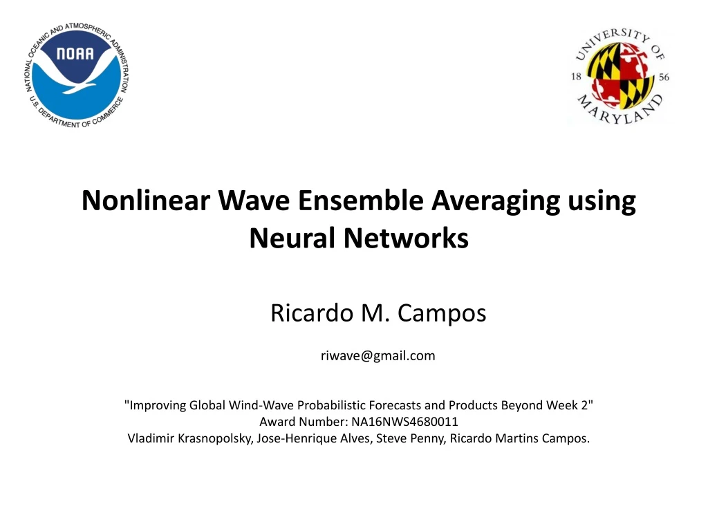
Nonlinear Wave Ensemble Averaging using Neural Networks Ricardo M. Campos riwave@gmail.com "Improving Global Wind-Wave Probabilistic Forecasts and Products Beyond Week 2" Award Number: NA16NWS4680011 Vladimir Krasnopolsky, Jose-Henrique Alves, Steve Penny, Ricardo Martins Campos.
Outline Quick introduction to GWES MLP Neural Networks applied to non-linear ensemble averaging First tests at single locations • NN Architectures • Tests with number of neurons, normalization etc • Error as afunction of Forecast time and Severity (Percentiles) NN spatial approach • NN Training Strategy • Spatial Distribution of Wind and Wave Climates • Assessment of GWES using NDBC buoys and Altimeters • Large sensitivity test: number of neurons, initialization, filtering • (1) GoM and (2) Global
Global Wave Ensemble System (GWES) The GWES was implemented in 2005 (Chen, 2006); 4 cycles per day; Resolution of 0.5 degree and 3 hours; Forecast range of 10 days; Total of 20 ensemble members plus a control member Forced by Global Ensemble Forecast System (GEFS) winds on WAVEWATCH III model (Tolman, 2016) Last major upgrade: 12/2015 Arithmetic Ensemble Mean:
MLP Neural Networks Multilayer perceptron model (MLP-NN) with hyperbolic tangent at the activation function. is the input and the output, and are the NN weights, and are the numbers of inputs and outputs respectively, and is the number of nonlinear basis functions (hyperbolic tangents, or ¨neurons¨) • Constructed based on Haykin(1999), Krasnopolsky (2013), and Krasnopolsky and Lin (2012) • NNs have been used in a wide variety of meteorology applications since the late 1980s (Key et al. 1989), from cloud classification (Bankert 1994), tornado prediction and detection (Marzban and Stumpf 1996; Lakshmananet al. 2005), damaging winds (Marzban and Stumpf 1998), hail size, precipitation classification, tracking storms (Lakshmanan et al. 2000), and radar quality control (Lakshmanan et al. 2007; Newman et al. 2013). AI techniques provide a number of advantages, including easily generalizing spatially and temporally, handling large numbers of predictor variables, integrating physical understanding into the models, and discovering additional knowledge from the data (McGovern et al., 2017).
MLP Neural Networks • Input variables: 10-meter wind speed (U10m), significant wave height (Hs), peak wave period (Tp), mean period, wave height of wind-sea, wave period of wind-sea; • Target variables: U10m, Hs, Tp from measurements; • Evaluated against buoy/altimeter observations during the training process; • 21 ensemble members (20 plus the control member) per variable, plus the sin and cosine of time; • Latitude and Longitude (sin,cos) are included as inputs during the regional analyses; • One NN per forecast time / forecast time as new degree of freedom; • Training (2/3) and test set (1/3); • Cross-validation with 3 cycles.
First tests at single locations ¨NNs are never used (or should never be used) for problems that can be solved using linear models¨ (Krasnopolsky, 2014) . NN models are indicated primarily to nonlinear problems; NN cannot deteriorate the EM! Residue (measurements - model) as the target variable
First tests at single locations The best NN model: 11 neurons at the intermediate layer Reduction of the error with increasing quantiles. Results of the NN simulation at the two Atlantic Ocean buoys. Curves of scatter indexes as afunction of quantiles; black: arithmetic mean of ensembles (EM); blue: NN-training set (buoy 41004), cyan: NN-validation set (buoy 41013). Solid lines indicate buoy 41004, and dashed lines buoy 41013.
NN spatial approach • Introduction of Lat/Lon as input variables instead of building one NN per grid point; • Increase of NN complexity, Krasnopolsky (2013): Different wind and wave climates. Correlation Coefficient Map of U10m and Hs
NN spatial approach - GOM • Simulation at the Gulf of Mexico. Sensitivity test: • Total of 12 different numbers of neurons • N [ 2, 5, 10, 15, 20, 25, 30, 35, 40, 50, 80, 200] • 8 different filtering windows • FiltW [ 0, 24, 48, 96, 144, 192, 288, 480] hours • 100 seeds for the random initialization • Separated NNs for specific forecast days, from Day 0 to Day 10 • Total of 105,600 NNs • NN training, 2/3 of inputs were selected for training and 1/3 for the test set, using a cross-validation scheme with 3 cycles • scikit-learn (python) to reduce computational cost • Six buoys appended to build the array with size 7913. NN is using sequential training
NN spatial approach - GOM Hs Day 5 Day 0 Day 10 Figure 9 - NBias, SCrmse, and CC according to equations 5, 8, and 11, resulted from the NN training tests on forecast Day 0
Results: NN spatial approach - GOM -Black: ensemble members -Red: ensemble mean -Cyan: control run --Green: NN
NN spatial approach - GOM Hurricane Hermine(September 02, 2016 – 00Z) Highest winds (1-minute sustained): 80 mph (36 m/s) Lowest pressure: 981 hPa
NN spatial approach - Global • NN modeling (whole globe) using altimeter data and joining all forecast times into the training (new degree-of-freedom); • 07/2016 – 07/2017 • 4 satellite missions: 15,993,200 measurements between 60°S and 60°N • 26 neurons [2-500], 10 seeds, and 3 datasets: total of 780 NNs U10 Hs
NN spatial approach - Global • Fday 0: sharp decay of the curve; 50 to 80 neurons • Fday 5: second minimum is found around 160 to 180 neurons. • Fday 10: best results using between 120 to 180 neurons. Higher RMSE for NNs with neurons equal to or less than 110. • The increasing scatter error of the surface winds at longer forecast ranges requires more complex NNs. Distance between the NN curves of training and test set. U10 Day 0 Day 5 Day 10 U10 U10 Day 0 Day 5 Day 10 Hs Hs Hs
NN spatial approach - Global • Results of 260 NNs, in terms of scatter error (y-axis) and systematic error (x-axis). • Left plots: training set in magenta and test set in green, compared to the control run (red square) and the arithmetic EM (cyan square) • Right plot: zoom-in the test set. Colorbar: number of neurons. Size of dots: normalized standard deviation of scatter error throughout different forecast ranges.
NN spatial approach - Global • “Best” selected based on three steps (ranking and excluding large errors). Final NN containing 140 neurons at the hidden layer. Weights/Biases and normalization parameters saved.
Conclusions • Wave Ensemble: Critical systematic and scatter errors are identified beyond the 6th- and 3rd- day forecasts, respectively. • The main advantage of the methodology using NNs at longer forecast ranges beyond four days. • Small number of neurons are sufficient to reduce the bias, while 35 to 50 neurons (GoM) produce the greatest reduction in both the scatter and systematic errors. • More complex NN models for global simulations incorporating the whole forecast range. • Systematic errors: very few neurons are sufficient to efficiently remove the bias, while more neurons are necessary to reduce the scatter error and improve the CC. • 60 to 80 neurons can minimize the errors of the nowcast but 120 (or more) neurons are necessary to properly address the errors of forecast day 10. • The operational implementation of the nonlinear ensemble averaging using NN is simple! • Next Step: ensemble of NNs based on Krasnopolsky and Lin (2012) - Control -.- EM -- NN
Obrigado! • Nonlinear Wave Ensemble Averaging using Neural Networks • Ricardo Campos, AOSC/UMD riwave@gmail.com ricardo.campos@centec.tecnico.ulisboa.pt • "Improving Global Wind-Wave Probabilistic Forecasts and Products Beyond Week 2" • Award Number: NA16NWS4680011 • Vladimir Krasnopolsky, Jose-Henrique Alves, Steve Penny, Ricardo Martins Campos.