Download
1 / 21
210 likes | 366 Vues
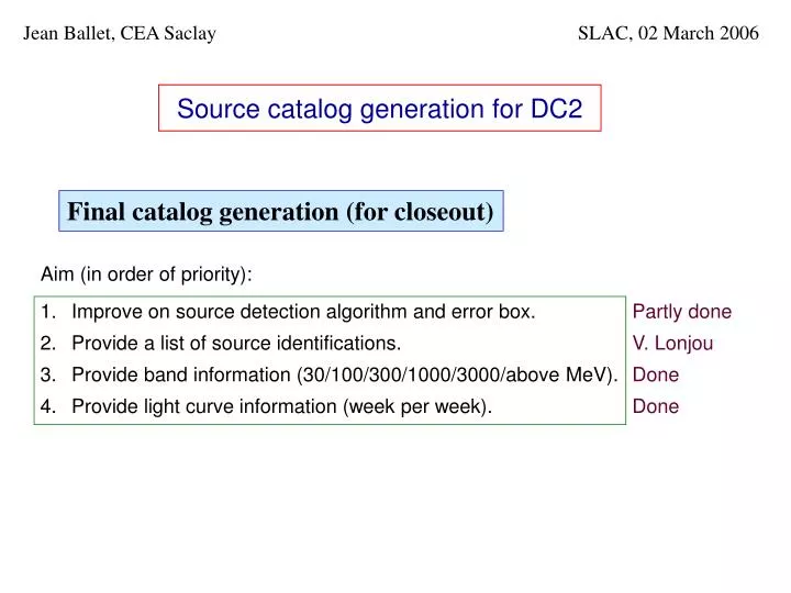
Source catalog generation for DC2. Jean Ballet, CEA Saclay. SLAC, 02 March 2006. Final catalog generation (for closeout). Aim (in order of priority):. Improve on source detection algorithm and error box. Provide a list of source identifications.

E N D
Source catalog generation for DC2 Jean Ballet, CEA Saclay SLAC, 02 March 2006 Final catalog generation (for closeout) Aim (in order of priority): Improve on source detection algorithm and error box. Provide a list of source identifications. Provide band information (30/100/300/1000/3000/above MeV). Provide light curve information (week per week). Partly done V. Lonjou Done Done
Catalog at DC2 kickoff Imaging step • Project sky onto 4 images (ARC for the poles and CAR for the Galactic plane) • Adjust diffuse model (background) in each projection separately • Run MR_filter + SExtractor independently on 3 bands (0.1 / 0.3 / 1 / 3 MeV) • Merge the 3 source lists into one, favoring high energy location Likelihood step • Restricted to events above 100 MeV (much faster, and finds most sources) • Pave the sky with Regions of Interest centered on no more than 10 sources • 5 iterations; Use DRMNGB, then final call to MINUIT to get errors • Threshold at Test Statistic = 25
Source catalog v2 • Improvement in the way MR_FILTER (source detection step) works in the extreme Poisson limit (very few photons). • Main gain: reduce number of spurious sources at high energy. Give illustration. • Add high energy band (> 3 GeV) to the source detection step. • 0.05° pixels, 4.5 sigma threshold, 0.17° error box. • Main gain: improve source position (and recover a few sources which are detectable only above 3 GeV). • 589 sources in output of the source detection step (imaging) • 380 sources validated by likelihood above Test Statistic = 25 • Distributed on Tuesday, May 9 (on regenerated data)
Source catalog v2 • 1 to 3 GeV vs 3 to 100 GeV toward (l,b) = (64,0); width is 40°; crosses are DC1 sources • Several rather bright spots at high energy do not appear below 3 GeV • Bright source to the left is clearly resolved above 3 GeV
Likelihood in energy bands Aim: Provide more energy information than a simple power-law index • The spectral index of all sources is fixed to the global (> 100 MeV) run • Each band (0.03 / 0.1 / 0.3 / 1 / 3 / 100 GeV) is treated independently • The diffuse emission normalizations (for extragalactic and Galactic components) are left free in each band and each Region of Interest • First run (DRMNGB optimizer) with sources outside the central region fixed to their best fit in the global run • Second run (MINUIT optimizer to get errors) with sources outside the central region fixed to the result of the first run (on a different RoI)
Likelihood in energy bands 2 Examples of bright sources (more than 100 sigma) • The dashed lines show the result of the global run • Remember that the global run started at 100 MeV • MRF0305 is a very nice power law • MRF0200’s slope probably adjusted largely within highest energy band
Likelihood in energy bands 3 Examples of faint sources (less than 10 sigma) • The dashed lines show the result of the global run • Remember that the global run started at 100 MeV • MRF0564 would have been much more significant starting at 30 MeV • MRF0118 is significant only in highest energy band
Likelihood in energy bands 4 Hardness ratios versus global slope • HRi = (Fi+1-Fi)/(Fi+1+Fi) • The full line is the theoretical value for a power law spectrum with 2 bands per decade • HR2 (stars) looks systematically larger than HR3 (diamonds)
Likelihood in energy bands 5 Color-color diagrams • Diamonds are bright sources (errors < 0.1), crosses are fainter sources • A power law spectrum should lie on the diagonal (hardness ratio independent of energy) • HR2 (horizontal) looks again systematically larger than HR3 (vertical)
Likelihood in time intervals Aim: Provide information on source variability • The energy selection is the same as in the global run (> 100 MeV) • The spectral index of all sources is fixed to the global run (spectral variations can be investigated outside the catalog context on bright sources where flux variations were detected) • The diffuse emission normalizations (for extragalactic and Galactic components) are fixed to the best fit values of the global run in each RoI (no reason why they should change) • Each one week interval is treated independently • First run (DRMNGB optimizer) with sources outside the central region fixed to their best fit in the global run • Second run (MINUIT optimizer to get errors) with sources outside the central region fixed to the result of the first run (on a different RoI)
Likelihood in time intervals 2 Examples of bright sources (more than 100 sigma) • Dashed and dotted lines show the flux returned on the full interval • MRF0059 is nicely constant • MRF0139 is one example of extreme variability
Likelihood in time intervals 3 Examples of faint sources (less than 10 sigma) • Dashed and dotted lines show the flux returned on the full interval • MRF0010 is nicely constant • MRF0397 is clearly variable • Error bars unreliable for not significant sources (linear)
Likelihood in time intervals 4 Variability search. Χ2Against constant value • Dashed line is the threshold 1% confidence level • 160 sources above that threshold (among 380) • Can apply other variability criteria
Final source catalog contents The official catalog format is given at https://confluence.slac.stanford.edu/display/ST/LAT+Source+Catalog+Contents • Source_Name (MRF + a number for internal reference), RA, DEC, Conf_95_SemiMajor (95% error radius)from all-sky source detection • Flux100 (100 MeV to 200 GeV) and error, Spectral_Index and error, Signif_Avg (in sigma units) from likelihood • Flux30_100, Flux100_300, Flux300_1000, Flux1000_3000, Flux3000_100000 (0.03 / 0.1 / 0.3 / 1 / 3 / 100 GeV) and errors from likelihood in bands • Flux_History(n), Unc_Flux_History(n) and History_Start(n+1) from likelihood in one week intervals (n=8 for DC2) We add for convenience: • L, B (Galactic coordinates) from all-sky source detection • Test_Statistic, Npred (number of photons above 100 MeV), Prefactor (ph/cm2/MeV/s at 100 MeV) from likelihood
Limitations The current catalog still has a number of serious limitations: • Initial source detection is still a place holder. See next session. • The threshold at which a source is considered significant (TS>25) is possibly too high. • The source position is imperfect (taken from highest energy band where source is detected). Need at least to combine energy bands. Could possibly use likelihood, but need to consider computing time. See also T. Burnett’s presentation. • The position error is extremely rough. Ideal would be to get it from likelihood, but computing time is very long. Started investigating formula relating position error to source significance in a given energy band. • The errors on flux and spectral index (from MINUIT) need to be assessed. Certainly very bad for not significant source fluxes in band and time pipelines.
Benchmarks Aim: Extrapolate hardware requirements to one year data (and more) Normalized to Linux PC at 3 GHz (we have 10 of those) • Computing time for imaging pipeline: relatively short (about 1 CPU day) • For main likelihood pipeline: 51.4 CPU days (32.8 for final iteration) • For energy band pipeline: 29.4 CPU days (13.1 + 8.9 + 4.5 + 2.2 + 0.7) • Time for time interval likelihood pipeline: 10.4 CPU days • Computing time is proportional to the number of events (unbinned likelihood). Binned likelihood could become competitive for longer intervals • Time is proportional to the number of sources left free in each RoI and to the number of RoIs, but also increases with the number of fixed sources (in ring around central part of RoI) Increases faster than number of sources
Source catalog generation for DC2 Jean Ballet, CEA Saclay GSFC, 31 May 2006 A reasonable DC2 catalog exists ! Outlook: Select initial source detection method (Seth’s talk tomorrow) Optimize source localization and error box determination Integrate source identification Build data base to support catalog work Devise a way to run the catalog pipeline on one year’s worth of data Think of adapting the catalog pipeline to transient source detection


![Planning contents of [DC2] LAT source catalog S. W. Digel Stanford Linear Accelerator Center](https://cdn2.slideserve.com/4043226/slide1-dt.jpg)