Download
1 / 43
430 likes | 535 Vues
Class Handout #9 (Chapter 6). Definitions. Two-Way Analysis of Variance (ANOVA).

E N D
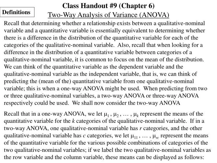
Class Handout #9 (Chapter 6) Definitions Two-Way Analysis of Variance (ANOVA) Recall that determining whether a relationship exists between a qualitative-nominal variable and a quantitative variable is essentially equivalent to determining whether there is a difference in the distribution of the quantitative variable for each of the categories of the qualitative-nominal variable. Also, recall that when looking for a difference in the distribution of a quantitative variable between categories of a qualitative-nominal variable, it is common to focus on the mean of the distribution. We can think of the quantitative variable as the dependent variable and the qualitative-nominal variable as the independent variable, that is, we can think of predicting the (mean of the) quantitative variable from one qualitative-nominal variable; this is when a one-way ANOVA might be used. When predicting from two or three qualitative-nominal variables, a two-way ANOVA or three-way ANOVA respectively could be used. We shall now consider the two-way ANOVA Recall that in a one-way ANOVA, we let 1 , 2 , … , k represent the means of the quantitative variable for the k categories of the qualitative-nominal variable. If in a two-way ANOVA, one qualitative-nominal variable has r categories, and the other qualitative-nominal variable has c categories, we let 11 , … , rc represent the means of the quantitative variable for the various possible combinations of categories of the two qualitative-nominal variables; if we label the two qualitative-nominal variables as the row variable and the column variable, these means can be displayed as follows:
Category #1 for Column Variable Category #2 for Column Variable Category #c for Column Variable Category #1 for Row Variable 11 12 1c 1* Category #2 for Row Variable 21 22 2c 2* Category #r for Row Variable r1 r2 rc r* *1 *2 *c ** The data for a two-way ANOVA consists of random observations of the quantitative variable for each possible combination of the categories of the two qualitative-nominal variables. Each of these possible combinations is called a cell of the table, and the corresponding means are called cell means. The double subscript indicates a specific combination of the categories, where the first subscript indicates the row variable category and the second subscript indicates the column variable category.
The means displayed outside the table at the end of each row represent row means, each one of which is the mean for the corresponding category of the row variable; the first subscript indicates the row variable category and the second subscript is an asterisk. The means displayed outside the table at the end of each column represent column means, each one of which is the mean for the corresponding category of the column variable; the first subscript is an asterisk and the second subscript indicates the column variable category. The mean displayed in the lower right corner outside the table represents the grand (overall) mean, which is the mean when all categories for both the row and column variable are combined together; both subscripts are asterisks. The following three questions are of interest in a two-way ANOVA: (1) (2) (3) Is there any statistically significant difference in the mean of the quantitative variable between categories of the row variable? Is there any statistically significant difference in the mean of the quantitative variable between categories of the column variable? Is there any statistically significant difference in the mean of the quantitative variable as a result of interaction between the row variable and column variable?
The first two questions can be addressed with two one-way ANOVAs, one for the row variable and one for the column variable. However, the third question, which concerns interaction, can only be addressed with a two-way ANOVA. An interaction is said to exist among the means for a row variable and a column variable when the difference between a pair of row means is not the same for each column category, and equivalently, the difference between a pair of column means is not the same for each row category. The differences in means between categories of the row variable and between categories of the column variable are called main effects; the differences in means resulting from interaction are interaction effects. Assumptions under which two-way ANOVA is appropriate are discussed on pages 160 and 161 of the textbook.
To illustrate the different types of differences among cell means that are possible, suppose the mean height (inches) of a plant is compared for two different types of soil (the row variable) labeled A and B, and for two different climates (the column variable) labeled Cool and Warm. The following tables of (population) means illustrate various combinations of effects which might exist: No Main Effects and No Interaction A Row Main Effect and No Interaction A Column Main Effect and No Interaction Cool Warm Cool Warm Cool Warm A B A B A B 20 20 20 20 20 30 20 20 25 25 20 30 Both Row and Column Main Effects and No Interaction Both Row and Column Main Effects and Interaction No Main Effects and Interaction Cool Warm Cool Warm Cool Warm A B A B A B 20 30 20 30 20 30 25 35 25 45 30 20
To answer each of the three questions of interest in a two-way ANOVA, a hypothesis test based on an f statistic is available. In each case the null hypothesis states that there is no difference in means from the corresponding effect. Each f statistic is a ratio of mean squares, similar to the one-way ANOVA f statistic. The sums of squares, degrees of freedom, mean squares, and f statistics can all be summarized into a two way ANOVA table which is often organized as follows, where n represents the total sample size: rc– 1 r– 1 c– 1 (r– 1)(c– 1) n–rc n– 1
The two-way ANOVA table is structured similar to the one-way ANOVA table and has a column for the different sources of variation, a column for degrees of freedom (df), a column for sums of squares (SS), and a column for mean squares (MS); also included are four f statistics with corresponding p-values. Each of the four f statistics is calculated by dividing the mean square in the corresponding row by the mean square in the Error row. The Overall Model row is concerned with the overall variation among cell means, and the f statistic in this row could be used in a hypothesis test to decide if there is at least one difference among the cell means (analogous to the hypothesis test in a one-way ANOVA); however, this hypothesis test is generally not of interest, since it does not focus on either the individual row and column variables or on the interaction between these variables. Observe that the degrees of freedom in this row is the number of cells rc minus one (1). The Rows row is concerned with the variation in cell means resulting from the row variable, and the f statistic in this row could be used in a hypothesis test to decide if there is at least one difference among the row means. Observe that the degrees of freedom in this row is the number of categories for the row variable r minus one (1).
The Columns row is concerned with the variation in cell means resulting from the column variable, and the f statistic in this row could be used in a hypothesis test to decide if there is at least one difference among the column means. Observe that the degrees of freedom in this row is the number of categories for the column variable c minus one (1). The Interaction row is concerned with the variation in cell means resulting from the interaction of the row variable and column variable, and the f statistic in this row could be used in a hypothesis test to decide if there is any statistically significant difference among the cell means resulting from interaction. Observe that the degrees of freedom in this row is the product of the degrees of freedom for the Rows row and the Columns row. The Error row is concerned with the variation within cells, that is, random variation; the mean square in this row is the denominator for each f statistic. Observe that the degrees of freedom in this row is the difference between the total sample size and the number of cells. The Total row is concerned with the total variation in the observed data when all cells are combined into one sample. Observe that the degrees of freedom in this row is the total sample size n minus one (1).
The degrees of freedom in the Overall Model row and in the Error row both add up to the degrees of freedom in the Total row. Also, the sum of squares in the Overall Model row and in the Error row both add up to the sum of squares in the Total row. The degrees of freedom in the Rows row, in the Columns row, and in the Interaction row all add up to the degrees of freedom in the Overall Model row. When the cell sizes in the data are all equal, then the sum of squares in the Rows row, in the Columns row, and in the Interaction row all add up to the sum of squares in the Overall Model row; however this may not be true, if the cell sizes are not all equal. The reason for this is because when the cell sizes in the data are all equal, then there is only one possible technique for computing the sums of squares in the Rows row, the Columns row, and the Interaction row; but when the cell sizes are not all equal, then there may be more than one technique for computing the sums of squares in the Rows row, the Columns row, and the Interaction row. In SPSS, the default technique for computing these sums of squares is called Type III sums of squares. The null hypotheses corresponding to the f tests in the Rows row, Columns row, and Interaction row of the two-way ANOVA table state respectively that there are no Row main effects, there are no Column main effects, and there are no Interaction effects. Generally speaking, if a researcher finds significant interaction, then describing the interaction effects is of primary interest, and whether or not there are main effects is of lesser interest. If a researcher finds no significant interaction, then whether or not there are main effects becomes of primary interest.
There are essentially three possible scenarios for the results in a two-way ANOVA: (1) Interaction effects and main effects are all found not to be statistically significant. In this scenario, the researcher would conclude that there is no difference in cell means, or in other words, the row variable and column variable are not significant in predicting the quantitative dependent variable. Hence, no further analysis would be necessary. (2) Interaction effects are found not to be statistically significant, but main effects are found to be statistically significant. In this scenario, the researcher would conclude that there is at least one difference in either row means, column means or both. Hence, further analysis would be necessary. When only two categories are compared, then describing the direction of the difference is necessary; when more than two categories are compared, then a multiple comparison procedure, such as those used when the f test in a one-way ANOVA is statistically significant, can be employed: Tukey’s Honestly Significant Difference (HSD) method, the Least Significant Difference (LSD) method, Bonferroni’s method, and Scheffe’s method are available when equal variances can be assumed, and Tamhane’s T2 method is available when unequal variances are assumed.
(3) Interaction effects are found to be statistically significant. Hence, further analysis would be necessary to describe the interaction effects. The researcher may or may not choose to consider main effects (using the procedures discussed in (2)), since these would now only be of secondary interest. To describe interaction, one possible method is Scheffe’s Multiple Comparison Procedure for Contrasts, which is performed in three steps: Go to the first exercise:
1. A 0.05 significance level is chosen for a two-way ANOVA to study the height to which wheat grows for two types of wheat, labeled D and E, and four different types of soil, labeled C, G, H, and T. From past experience, it can be assumed that the wheat height is normally distributed.. A random sample of heights is recorded in inches for each possible combination of wheat type and soil type with the following results: Soil Type C Soil Type G Soil Type H Soil Type T Wheat Type D 37.4 35.1 41.8 44.1 46.4 40.0 42.2 38.8 47.4 33.0 31.1 27.1 Wheat Type E 31.8 28.5 36.6 35.6 42.6 38.5 27.9 22.9 26.0 30.8 36.9 34.3 The data has been stored in the SPSS data file wheat. Use the Analyze>General Linear Model> Univariate options in SPSS to display the Univariate dialog box. Select the variable height for the Dependent Variable slot, and select the variables wheattype and soiltype for the Fixed Factor(s) section. Click on the Post Hoc button to display the Univariate: Post Hoc Multiple Comparisons for Observed Means dialogue box. From the list in the Factor(s) section on the left, select the variables wheattype and soiltype for the Post Hoc Tests for section on the right. Select the Bonferroni multiple comparison procedure in the Equal Variances Assumed section. Click on the Continue button to return to the Univariate dialog box. (a)
Click on the Options button to display the Univariate: Options dialogue box. From the list in the Factor(s) and Factor Interactions section on the left, select (OVERALL), wheattype, soiltype, and wheattype*soiltype for the Display Means for section on the right. Select Estimates of effect size and Homogeneity tests in the Display section. Click on the Continue button to return to the Univariate dialog box. Click on the Plots button to display the Univariate: Profile Plots dialogue box. From the list in the Factor(s) section on the left, select wheattype for the Horizontal Axis slot on the right, and select soiltype for the Separate Lines slot on the right; then, click the Add button to add this plot to the Plots section. Now, from the list in the Factor(s) section on the left, select soiltype for the Horizontal Axis slot on the right, and select wheattype for the Separate Lines slot on the right; then, click the Add button to add this plot to the Plots section. Click on the Continue button to return to the Univariate dialog box. Click on the OK button, after which results are displayed in an SPSS output viewer window.
Comment on what the results of Levene’s test tells us about the equal variance assumption for a two-way ANOVA. (b) Levene’s test is not statistically significant at the 0.05 level (f7,16 = 0.172, p = 0.988). Thus, we conclude that the equal variance assumption for a two-way ANOVA is satisfied.
1.-continued Looking at the ANOVA table displayed on the SPSS output, explain which of the three possible scenarios for the results in a two-way ANOVA have occurred with this data. (c) We find from the ANOVA table that there are statistically significant interaction effects at the 0.05 level (f3,16 = 9.282, p = 0.001). We also find that there are statistically significant main effects for both wheat type (f1,16 = 18.261, p = 0.001) and soil type (f3,16 = 7.609, p = 0.002), but describing the interaction is the primary interest. Complete the analysis of this two-way ANOVA data according to the scenario for the results in part (c). (d) Since we have concluded that there are significant interaction effects, we need to describe the interaction effects, and we shall use Scheffe’s Multiple Comparison Procedure for Contrasts to do this. Return to the description of Scheffe’s Multiple Comparison Procedure for Contrasts at the beginning of the handout:
(3) Interaction effects are found to be statistically significant. Hence, further analysis would be necessary to describe the interaction effects. The researcher may or may not choose to consider main effects (using the procedures discussed in (2)), since these would now only be of secondary interest. To describe interaction, one possible method is Scheffe’s Multiple Comparison Procedure for Contrasts, which is performed in three steps: Note: we shall let yij represent the cell mean in the data for row i and column j. Column #g Column #h Find the absolute value of each contrast involving cell means of the form Step 1: Row #i yig yih yig yih – – yjg + yjh = yig yih – – yjg – yjh = Row #j yjg yjh yih yig yjg – – – yjh
Step 2: Step 3: Declare a contrast to be statistically significant if it has an absolute value larger than (r– 1)(c– 1)(f(r–1)(c–1) , n–rc ; )(MSE)(1/nig + 1/nih + 1/njg + 1/njh) If all cell sizes are equal, say to m, then this quantity reduces to 4 / m . This is the tabled f value defining the rejection region in the test concerning interaction. Mean Square Error with interaction terms in the model Summarize the results by describing the interaction effect corresponding to each statistically significant contrast. There are basically two types of interaction effects which can occur: One is where the difference between means is in the same direction in two different categories but is of a different magnitude in the two categories. The other is where the difference between means is in opposite directions in two different categories. Assumptions under which two-way ANOVA is appropriate are discussed on pages 160 and 161 of the textbook.
From the SPSS output, we construct the following table of cell means: Soil Type C Soil Type G Soil Type H Soil Type T Wheat Type D 42.8 38.1 43.5 30.4 Wheat Type E 32.3 38.9 25.6 34.0 absolute value of contrasts: 11.4 1.2 | 38.1 – 42.8 – 32.3 + 25.6 | = | 38.1 – 43.5 – 32.3 + 38.9 | = 12.6 9.4 | 43.5 – 42.8 – 38.9 + 25.6 | = | 38.1 – 30.4 – 32.3 + 34.0 | = 20.8 8.2 | 42.8 – 30.4 – 25.6 + 34.0 | = | 43.5 – 30.4 – 38.9 + 34.0 | = = 12.38 (1) (3) (3.24) (11.829) (1/3 + 1/3 + 1/3 + 1/3) With = 0.05, we conclude the following: The amount that mean height with soil type G exceeds mean height with soil type H is larger with wheat type E than with wheat type D. For wheat type D, mean height with soil type H is larger than mean height with soil type T; for wheat type E, this difference is in the opposite direction.
The conclusions were stated in terms of comparing the differences between soil types for the two wheat types. Alternatively, the conclusions can be stated in terms of comparing the differences between wheat types for two soil types.
From the SPSS output, we construct the following table of cell means: Soil Type C Soil Type G Soil Type H Soil Type T Wheat Type D 42.8 38.1 43.5 30.4 Wheat Type E 32.3 38.9 25.6 34.0 absolute value of contrasts: 11.4 1.2 | 38.1 – 42.8 – 32.3 + 25.6 | = | 38.1 – 43.5 – 32.3 + 38.9 | = 12.6 9.4 | 43.5 – 42.8 – 38.9 + 25.6 | = | 38.1 – 30.4 – 32.3 + 34.0 | = 20.8 8.2 | 42.8 – 30.4 – 25.6 + 34.0 | = | 43.5 – 30.4 – 38.9 + 34.0 | = = 12.38 (1) (3) (3.24) (11.829) (1/3 + 1/3 + 1/3 + 1/3) With = 0.05, we conclude the following: The amount that mean height with wheat type D exceeds mean height with wheat type E is larger with soil type H than with soil type G. For soil type H, mean height with wheat type D is larger than mean height with wheat type E; for soil type T, this difference is in the opposite direction.
1.-continued Although describing the interaction is of primary interest, significant main effects for both wheat type and soil type were found. From Bonferroni’s multiple comparison method with = 0.05, we conclude the following: The mean height is greater with Soil Type G than with Soil Type C (p = 0.049). The mean height is greater with Soil Type G than with Soil Type H (p = 0.017). The mean height is greater with Soil Type G than with Soil Type T (p = 0.002). With = 0.05, we also conclude that mean height is greater with Wheat Type D than with Wheat Type E (p = 0.001).
The “Partial Eta Squared” column of the ANOVA table on the SPSS output displays the proportion of total variance in the dependent variable (height) accounted for by each independent variable: Wheat Type, Soil Type, and Interaction between Wheat Type and Soil Type. Find the percent of total variance accounted for by each of these three independent variables. (e) Wheat Type accounts for 53.3% of the variance in height, Soil Type accounts for 58.8% of the variance in height, and Interaction between Wheat Type and Soil Type accounts for 63.5% of the variance in height. Observe that the SPSS output displays a warning that no post hoc tests were performed for type of wheat because there were fewer than three groups. Explain why are post hoc tests unnecessary when fewer than three groups are being compared. (f) When only two groups are being compared, then only one statistically significant difference is possible, making multiple comparison unnecessary.
2. Mean yearly income ($1000s) for voters who are employed full time in a state is being studied. A 0.05 significance level is chosen for a two-way ANOVA to compare mean yearly income for males and females and for three areas of residence: rural, suburban, and urban. The random sample of voters to be used consists of those in the data set of Exercise #1 on Class Handout #1; this data is stored in the SPSS data file survey. (Note: Examination of the data will reveal that each cell size is 5.) Use the Analyze>Descriptive Statistics> Explore options in SPSS to display the Explore dialog box. Select the variable income for the Dependent List section, and make certain that the option Both has been selected in the Display section. Click on the Plots button to display the Explore: Plots dialogue box. Select the option Histogram and the option Normality plots with tests.Click on the Continue button to return to the Explore dialog box. Click on the OK button, after which results are displayed in an SPSS output viewer window. (a) After finding on the SPSS output the descriptive statistics for income concerning skewness and kurtosis, the histogram and box plot, and the normal probability plots, comment on whether the normality assumption for a two-way ANOVA appears to be satisfied. (b)
Neither the skewness coefficient or the kurtosis coefficient is more than two standard errors away from zero. Both the histogram and the box plot show some positive skewness, but it does not seem to be severe, and there are no outliers. The normal probability plots appear to show some non-normality in the distribution of income, but since it does not appear to be severe, we can reasonably conclude that the two-way ANOVA is appropriate.
2.-continued Use the Analyze>General Linear Model> Univariate options in SPSS to display the Univariate dialog box. Select the variable income for the Dependent Variable slot, and select the variables sex and residnce for the Fixed Factor(s) section. Click on the Post Hoc button to display the Univariate: Post Hoc Multiple Comparisons for Observed Means dialogue box. From the list in the Factor(s) section on the left, select the variables sex and residnce for the Post Hoc Tests for section on the right. Select the Bonferroni multiple comparison procedure in the Equal Variances Assumed section. Click on the Continue button to return to the Univariate dialog box. Click on the Options button to display the Univariate: Options dialogue box. From the list in the Factor(s) and Factor Interactions section on the left, select (OVERALL), sex, residnce, and sex*residnce for the Display Means for section on the right. Select Estimates of effect size and Homogeneity tests in the Display section. Click on the Continue button to return to the Univariate dialog box. (c)
Click on the Plots button to display the Univariate: Profile Plots dialogue box. From the list in the Factors section on the left, select sex for the Horizontal Axis slot on the right, and select residnce for the Separate Lines slot on the right; then, click the Add button to add this plot to the Plots section. Now, from the list in the Factors section on the left, select residnce for the Horizontal Axis slot on the right, and select sex for the Separate Lines slot on the right; then, click the Add button to add this plot to the Plots section. Click on the Continue button to return to the Univariate dialog box. Click on the OK button, after which results are displayed in an SPSS output viewer window. Comment on what the results of Levene’s test tells us about the equal variance assumption for a two-way ANOVA. (d) Levene’s test is not statistically significant at the 0.05 level (f5,24 = 0.941, p = 0.473). Thus, we conclude that the equal variance assumption for a two-way ANOVA is satisfied.
2.-continued Looking at the ANOVA table displayed on the SPSS output, explain which of the three possible scenarios for the results in a two-way ANOVA have occurred with this data. (e) We find from the ANOVA table that there are no statistically significant interaction effects at the 0.05 level (f5,24 = 2.702, p = 0.087). Even though the interaction is not statistically significant at the chosen 0.05 level, the fact that the p-value is less than 0.10 will make some researchers think that perhaps there could be statistical significance in a future study with a larger sample size. We find that there are statistically significant main effects for both sex (f1,24 = 15.086, p = 0.001) and residence (f2,24 = 6.541, p = 0.005). Since only the main effects are statistically significant, identifying these significant main effects is of primary interest.
2.-continued Complete the analysis of this two-way ANOVA data according to the scenario for the results in part (e). (f) Since we have concluded that there are significant main effects, we need to identify significant differences in row means and in column means. The row variable sex has only two categories, and since we concluded that the difference in mean yearly income between sexes was different, we just need to identify the direction of the difference. The column variable area of residence has three categories, and since we concluded that there is at least one difference in mean yearly income, we need to use multiple comparison to identify the differences. We shall use Bonferroni’s method to do this.
2.-continued From Bonferroni’s multiple comparison method with = 0.05, we conclude the following: The mean yearly income is greater in the suburban area than in the rural area (p = 0.010). The mean yearly income is greater in the urban area than in the rural area (p = 0.020). With = 0.05, we also conclude that mean yearly income is greater for males than for females (p = 0.001).
The “Partial Eta Squared” column of the ANOVA table on the SPSS output displays the proportion of total variance in the dependent variable (income) accounted for by each independent variable: sex, residence, and interaction between sex and residence. Find the percent of total variance accounted for by each of these three independent variables. (g) Sex of the voter accounts for 38.6% of the variance in yearly income, area of residence accounts for 35.3% of the variance in yearly income, and Interaction between sex and residence accounts for 18.4% of the variance in yearly income. Observe that the SPSS output displays a warning that no post hoc tests were performed for sex because there were fewer than three groups. Explain why are post hoc tests unnecessary when fewer than three groups are being compared. (h) When only two groups are being compared, then only one statistically significant difference is possible, making multiple comparison unnecessary.
3. Read the “INTRODUCTION” and “TWO-WAY ANALYSIS OF VARIANCE” sections of Chapter 6. Open the SPSS data file Job Satisfaction. (a) In the “PRACTICAL EXAMPLE” section, read the discussion for assumptions number 1 to 4 in the subsection “Hypothesis Testing”; then, use the Analyze> Descriptive Statistics> Explore options in SPSS to obtain the information in Table 6.2 and the graphs in Figure 6.1. (Table 6.3 displayed in this subsection can be obtained from work to be done in the subsection which follows.) (b) In the “PRACTICAL EXAMPLE” section, read the subsection “How to Use SPSS to Run Two-Way ANOVA”, and follow the instructions with SPSS, which should produce the output displayed in Table 6.4 to Table 6.9 and in Figure 6.2. Compare the syntax file commands generated by the output with those shown on page 167 of the textbook. Read the remaining portion of Chapter 6.