Download
1 / 61
610 likes | 735 Vues
COMP171 Fall 2006. Graphs. Slides from HKUST. Graphs. Extremely useful tool in modeling problems Consist of: Vertices Edges. Vertices can be considered “sites” or locations. Edges represent connections. D. E. C. A. F. B. Vertex. Edge. Application 1. Air flight system.

E N D
COMP171 Fall 2006 Graphs Slides from HKUST
Graphs • Extremely useful tool in modeling problems • Consist of: • Vertices • Edges Vertices can beconsidered “sites”or locations. Edges represent connections. D E C A F B Vertex Edge
Application 1 Air flight system • Each vertex represents a city • Each edge represents a direct flight between two cities • A query on direct flights = a query on whether an edge exists • A query on how to get to a location = does a path exist from A to B • We can even associate costs to edges (weighted graphs), then ask “what is the cheapest path from A to B”
Application 2: The Minimum Spanning Tree • Weighted graphs: the cost to connect A and B by a communication line is 7 units. • Can we build a communication network so that every two vertex are connected with the minimum costs?
Application 3 Wireless communication • Represented by a weighted complete graph (every two vertices are connected by an edge) • Each edge represents the Euclidean distance dij between two stations • Each station uses a certain power i to transmit messages. Given this power i, only a few nodes can be reached (bold edges). A station reachable by i then uses its own power to relay the message to other stations not reachable by i. • A typical wireless communication problem is: how to broadcast between all stations such that they are all connected and the power consumption is minimized.
{a,b} {a,c} {b,d} {c,d} {b,e} {c,f} {e,f} Definition • A graph G=(V, E) consists a set of vertices, V, and a set of edges, E. • Each edge is a pair of (v, w), where v, w belongs to V • If the pair is unordered, the graph is undirected; otherwise it is directed • Consider a simple graph where E is not a multiple set and it doesn’t contain elements of the form {x,x}, i.e. no loop and no multiple edges. An undirected graph
Terminology • If v1 and v2 are connected, they are said to be adjacent vertices • v1 and v2 are endpoints of the edge {v1, v2} • If an edge e is connected to v, then v is said to be incident one. Also, the edge e is said to be incident onv. • The number of incident edges on v is the degree of v. • Basic theorem: Let n be the number (size) of vertices and m be the number of edges, then
Path between Vertices • A path is a sequence of vertices (v0, v1, v2,… vk) such that: • For 0 ≤ i < k, {vi, vi+1} is an edge Note: a path is allowed to go through the same vertex or the same edge any number of times! • The length of a path is the number of edges on the path • A closed path is a path with the same starting and ending vertex.
Types of paths • A path is simple if and only if it does not contain a vertex more than once. • A closed path is a cycle if and only if it has no repeated edges. • A graph is connected if there is a path between any two vertices. • A tree is graph that is connected and has no cycles.
Path Examples Are these paths? Any cycles? What is the path’s length? • {a,c,f,e} • {a,b,d,c,f,e} • {a, c, d, b, d, c, f, e} • {a,c,d,b,a} • {a,c,f,e,b,d,c,a}
Directed Graph • A graph is directed if direction is assigned to each edge. • Directed edges are denoted as arcs. • Arc is an ordered pair (u, v) • Recall: for an undirected graph • An edge is denoted {u,v}, which actually corresponds to two arcs (u,v) and (v,u)
Indegree and Outdegree • Since the edges are directed, we need to consider the arcs coming “in” and going “out” • Thus, we define terms Indegree(v), and Outdegree(v) • Each arc(u,v) contributes count 1 to the outdegree of u and the indegree of v
Directed Acyclic Graph • A directed path is a sequence of vertices (v0, v1, . . . , vk) • Such that (vi, vi+1) is an arc • A directed cycle is a directed path such that the first and last vertices are the same. • A directed graph is acyclic if it does not contain any directed cycles
3 6 8 0 7 2 9 1 5 4 Example Is it a DAG?
Directed Graphs Usage • Directed graphs are often used to represent order-dependent tasks • That is we cannot start a task before another task finishes • We can model this task dependent constraint using arcs • An arc (i,j) means task j cannot start until task i is finished • Clearly, for the system not to hang, the graph must be acyclic j Task j cannot start until task i is finished i
University Example • CS departments course structure 104 180 151 171 221 342 252 201 211 251 271 M111 M132 231 272 361 381 303 343 341 327 334 336 362 332 Any directed cycles? How many indeg(171)? How many outdeg(171)?
3 6 8 0 7 2 9 1 5 4 Topological Sort • Topological sort is an algorithm for a directed acyclic graph • Linearly order the vertices so that the linear order respects the ordering relations implied by the arcs For example: 0, 1, 2, 5, 9? 0, 4, 5, 9? 0, 6, 3, 7 ?
Topological Sort Algorithm • Observations • Starting point must have zero indegree • If it doesn’t exist, the graph would not be acyclic • Algorithm • A vertex with zero indegree is a task that can start right away. So we can output it first in the linear order • If a vertex i is output, then its outgoing arcs (i, j) are no longer useful, since tasks j does not need to wait for i anymore- so remove all i’s outgoing arcs • With vertex i removed, the new graph is still a directed acyclic graph. So, repeat step 1-2 until no vertex is left.
Graph Representation • Two popular computer representations of a graph. Both represent the vertex set and the edge set, but in different ways. • Adjacency Matrix Use a 2D matrix to represent the graph • Adjacency List Use a 1D array of linked lists
Adjacency Matrix • The graph G = (V, E) can be represented by a table, or a matrix M = (aij)n×n aij = 1 iff (vi, vj) ∈E, assuming V = {v1, …, vn}.
Adjacency Matrix • 2D array A[0..n-1, 0..n-1], where n is the number of vertices in the graph • Each row and column is indexed by the vertex id • e,g a=0, b=1, c=2, d=3, e=4 • A[i][j]=1 if there is an edge connecting vertices i and j; otherwise, A[i][j]=0 • The storage requirement is Θ(n2). It is not efficient if the graph has few edges. An adjacency matrix is an appropriate representation if the graph is dense: |E|=Θ(|V|2) • We can detect in O(1) time whether two vertices are connected.
Adjacency List • The graph G = (V, E) can be represented by a list of vertices and a list of its adjacent vertices for each vertex. Adjacent vertices for each vertex: a: {c, d, e} b: { } c: {a, e} d: {a ,e} e: {a, d, c}
Adjacency List • If the graph is not dense, in other words, sparse, a better solution is an adjacency list • The adjacency list is an array A[0..n-1] of lists, where n is the number of vertices in the graph. • Each array entry is indexed by the vertex id • Each list A[i] stores the ids of the vertices adjacent to vertex i
0 8 2 9 1 7 3 6 4 5 Adjacency Matrix Example
0 8 2 9 1 7 3 6 4 5 Adjacency List Example
Storage of Adjacency List • The array takes up Θ(n) space • Define degree of v, deg(v), to be the number of edges incident to v. Then, the total space to store the graph is proportional to: • An edge e={u,v} of the graph contributes a count of 1 to deg(u) and contributes a count 1 to deg(v) • Therefore, Σvertex vdeg(v) = 2m, where m is the total number of edges • In all, the adjacency list takes up Θ(n+m) space • If m = O(n2) (i.e. dense graphs), both adjacent matrix and adjacent lists use Θ(n2) space. • If m = O(n), adjacent list outperform adjacent matrix • However, one cannot tell in O(1) time whether two vertices are connected
Adjacency List vs. Matrix • Adjacency List • More compact than adjacency matrices if graph has few edges • Requires more time to find if an edge exists • Adjacency Matrix • Always require n2 space • This can waste a lot of space if the number of edges are sparse • Can quickly find if an edge exists
Representations for Directed Graphs • The adjacency matrix and adjacency list can be used
3 6 8 0 7 2 9 1 5 4 Topological Sort, the algorithm 1) Choose a vertex v of indegree 0 (what about there are several such vertices?) and output v; 2) Modify the indegree of all the successor of v by subtracting 1; 3) Repeat the above process until all vertices are output.
Topological Sort Find all starting points Reduce indegree(w) Place new startvertices on the Q
Time Complexity of Topological Sorting (Using Adjacency Lists) • We never visited a vertex more than one time • For each vertex, we had to examine all outgoing edges • Σ outdegree(v) = m • This is summed over all vertices, not per vertex • So, our running time is exactly • O(n + m) How about the complexity using adjacency matrix?
Graph Traversal • Application example • Given a graph representation and a vertex s in the graph • Find all paths from s to other vertices • Two common graph traversal algorithms • Breadth-First Search (BFS) • Find the shortest paths in an unweighted graph • Depth-First Search (DFS) • Topological sort • Find strongly connected components
0 8 2 9 1 7 3 6 4 5 2 s 1 1 2 1 2 2 1 BFS and Shortest Path Problem • Given any source vertex s, BFS visits the other vertices at increasing distances away from s. In doing so, BFS discovers paths from s to other vertices for unweighted graphs. • What do we mean by “distance”? The number of edges on a path from s Example Consider s=vertex 1 Nodes at distance 1? 2, 3, 7, 9 Nodes at distance 2? 8, 6, 5, 4 Nodes at distance 3? 0
BFS Algorithm // flag[ ]: visited table Why use queue? Need FIFO
Time Complexity of BFS(Using Adjacency List) • Assume adjacency list • n = number of vertices m = number of edges O(n + m) Each vertex will enter Q at most once. Each iteration takes time proportional to 1 + deg(v).
Running Time • Recall: Given a graph with m edges, what is the total degree? • The total running time of the while loop is: this is summing over all the iterations in the while loop! • See ds.soj.me for practice. Σvertex v deg(v) = 2m O( Σvertex v (1 + deg(v)) ) = O(n+m)
Time Complexity of BFS(Using Adjacency Matrix) • Assume adjacency matrix • n = number of vertices m = number of edges O(n2) Finding the adjacent vertices of v requires checking all elements in the row. This takes linear time O(n). Summing over all the n iterations, the total running time is O(n2). So, with adjacency matrix, BFS is O(n2) independent of the number of edges m. With adjacent lists, BFS is O(n+m); if m=O(n2) like in a dense graph, O(n+m)=O(n2).
Dijkstra’s Shortest Path Algorithm(A Greedy Algorithm) • Assume the weighted graph has no negative weights (Why?). • Single source shortest path problem:find all the shorted paths from source s to other vertices. • Basic idea: list all the shortest paths from the source s • Dijkstra’s algorithm is a greedy algorithm, and the correctness of the algorithm can be proved by contradiction. • Time complexity O(|V|2).
Example • Ideas of the algorithm (Dijkstra): enumerate the shortest paths from the source to other vertices in increasing order. Basic observations: • If (s, u,..,v, w) is a shorted path from s to w, then (s,u,…,v) must be a shortest path form s to v. • The shortest path from s to v should be the shortest one among those paths from s to v which only go through known shortest paths. Method: On every vertex v maintain a pair (known, dist), known: whether the shortest distance from the source s to v is known, dist: the shortest distance from s through known vertices. 1. To list the next shortest path, find the vertex v with smallest dist, and mark v as known. 2. update labels for the successors of v. 3. goto 1 until all the shortest paths are found.
Example Method: Mark every vertex v with a pair (known, dist), known: whether the shortest distance from the source s to v is known, dist: the shortest distance from s through known vertices. • Starting with : mark every vertex v with (F, w(s,v)), s with (T, 0). • The next shortest distance from s is the one with the smallest dist among vertices (F, dist), and mark that vertex v with T. • Update dist of those unknown vertices which are adjacent to v ; • Goto 2 until all vertices are known.
Dijkstra’s Algorithm Dijkstra(G, s): Input: s is the source Output: mark every vertex with the shortest distance from s. for every vertex v { set v (F, weight(s,v)) } set s(T, 0); while ( there is a vertex with (F, _)) { find the vertex v with the smallest distvamong (F, dist) set v(T, distv) for every w(F, dist) adjacent to v { if(distv+ weight(v,w) < dist) set w(F, distv + weight(v,w)) } } Linear, but can be improved by using heaps. Can you add more information to get the shortest paths?
Running Time • If we use a vector to store “dist” information for all vertices, then finding the smallest value takes O(|V|) time, and the total updating takes O(|E|) time, and the running time is O(|V|2). • If we use a binary heap to store “dist” information, the finding the smallest takes O(log|V|) time and every updating also takes O(log|V|) time, so the total running time is O(|V|) + O(|V|log|V|) +O(|E|log|V|) = O(|E|log|V|).
Greedy algorithms A greedy algorithm is used in optimization problems. It makes the local optimal choice at each stage with the hope of finding the global optimum. • Example 1. Make 87yuan using the fewest possible bills. Using greedy algorithm, one can choose • 50, 20, 10, 5, 2, and this is the optimal solution. • Example 2. Make 15 krons, where available bills are 1, 7 and 10. • Using greedy algorithm, the solution is 10, 1,1,1,1,1. • The best solution is 7, 7, and 1.
Proving Its Correctness • The greedy approach leads to: • simple and intuitive algorithms • efficient algorithms • But , it does not always lead to an optimal solution. • Since the greedy approach doesn’t assure the optimality of the solution we have to analyze for each particular problem if the algorithm leads to an optimal solution.
Proving the correctness of the algorithm • We can prove that the distance recorded in distance is the length of the shortest path from source to v. • Prove: when v is choosen and marked with (T, dist), dist is the shortest path from 0 to v . distance[x]<distance[v] And x must be in S Notice that the assumption is the weight is positive. Red vertices are marked with T, x is the first unknown vertex on the shortest path from 0 to v
Dijkstra • Shortest path algorithm paper • EWD hand writing notes • http://www.cs.utexas.edu/users/EWD/
Minimum Spanning Trees • Definition of minimum spanning trees for undirected, connected, weighted graphs. • Prim’s algorithm, a greedy algorithm. • Basic observation: G=(V,E), for any A V, if an edge e has the smallest weight connection A and V-A, then e is in a MST. • A local optimal choice is also a global optimal choice.
Prim’s Algorithm • Method: Build the MST by adding vertices and edges one by one staring with one vertex. At some stage, let A be the set of the vertices that are already added, V-A be the set of the remaining vertices that are not added. • Find the smallest weighted edge e = (u,v), that connects A and V-A, that is, e has the smallest weight among those edges with uA and v V-A. • Now add vertex v to A and edge (u,v) to the MST. • Repeat step 1 and 2 above until A=V.
Prim’s Algorithm --An Example • 1. Starting from a node, 0; • 2. Add a vertex v and an edge (0,v) which has a weight as small as possible 3. Add a vertex u such that an edge connecting u and {0,v} has a weight as small as possible; 4. Repeat the process until all vertices are added.