Download
1 / 33
330 likes | 335 Vues
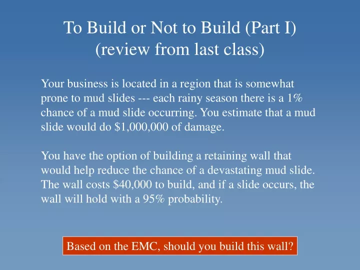
To Build or Not to Build (Part I) (review from last class). Your business is located in a region that is somewhat prone to mud slides --- each rainy season there is a 1% chance of a mud slide occurring. You estimate that a mud slide would do $1,000,000 of damage.

E N D
To Build or Not to Build (Part I)(review from last class) Your business is located in a region that is somewhat prone to mud slides --- each rainy season there is a 1% chance of a mud slide occurring. You estimate that a mud slide would do $1,000,000 of damage. You have the option of building a retaining wall that would help reduce the chance of a devastating mud slide. The wall costs $40,000 to build, and if a slide occurs, the wall will hold with a 95% probability. Based on the EMC, should you build this wall?
To Build or Not to Build (Part II) You also have the option of having a test done to determine whether or not a slide will occur in your specific location. The test costs $3,000 and has the following accuracies: P(test positive | slide occurs) = 0.90 P(test negative | slide doesn’t occur) = 0.85 If you choose the test, then, based on the result of the test, you will either build or not build. Based on the EMC, what should your decision strategy be?
Risk in the Mud Slide Example • EMC says to not build the wall • Is this the right decision? • There’s still a 1% chance of losing everything ($1,000,000 --- not to mention the business) Given that you build the wall without testing, what is the probability that you’ll lose everything? Given that you choose the test, what is the probability that you’ll lose everything? Answers can be gotten from the tree…
Slide Doesn’t Hold Given that you build the wall without testing, what is the probability that you’ll lose everything? With the given situation, there is one path (or sequence of events and decisions) that leads to losing everything: Build w/o testing 0.05 given 0.01 P( losing everything | build w/o testing ) = 0.01 * 0.05 = 0.0005
Pos Build Slide Doesn’t Hold Neg Don’t Build Slide Given that you choose the test, what is the probability that you’ll lose everything? With the given situation, there are two paths (or sequences of events and decisions) that lead to losing everything: Test given 0.0571 0.05 0.1575 Test given 0.0012 0.8425 P( first path ) = 0.1575 * 0.0571 * 0.05 = 0.00045 P( second path ) = 0.8425 * 0.0012 = 0.00101 P( losing everything | testing ) = 0.00045 + 0.00101 = 0.00146
Summarizing our choices… Now which looks best? Perhaps testing is best because it balances both EMC and risk
Risk in Decision Analysis Problems • There are two ways to talk about risk in DA: • Standard deviation (we’ll talk about this soon) • “Negative outcome” analysis • Consider the probability of most negative outcome • And balance it with EMC Use negative outcome analysis on Homework #3
Sensitivity Analysis We have analyzed the mud slide situation with the parameter that the wall costs $40,000. You may wonder: would my decision change if the wall cost $35,000 or $45,000 or …? Sensitivity analysis is the investigation of how changes in the problem data affect the problem outcome “How sensitive is the outcome to changes in the data?”
Discrete Random Variables discrete = consisting of unconnected, distinct parts Think about a chance event with a finite number of outcomes… A discrete random variable is an assignment of numbers, or values, to a collection of MECE events MECE = mutually exclusive, collectively exhaustive
1.0 3.5 -2.0 3.5 A B C D • Usually, a capital letter, like X, is used to denote the random variable • The assigned numbers mean something in the context of the situation (above is just an example) P( X = -2.0 ) = P(C) New ideas for probability: P( X = 1.0 ) = P(A) P( X = 3.5 ) = P(B) + P(D)
Examples of Discrete Random Variables X = 1 if Heads X = 0 if Tails P( X = 0 ) = P( X = 1 ) = 0.5 Heads and Tails X = 1000 if No Rain P( X = 1000 ) = 0.3 X = 500 if Rain P( X = 500 ) = 0.7 J&J Flea Market Saturday Y = 700 if No Rain P( Y = 700 ) = 0.7 Y = 350 if Rain P( Y = 350 ) = 0.3 J&J Flea Market Sunday
Examples of Discrete Random Variables X = price of stock P( X = 50 ) = ??? Stock 100 items produced per day X = number of defective items P( X = 20 ) = ??? P( X 5 ) = ??? P( X = 0 ) = ??? Assembly Line Random variables are often talked about in terms of the assigned values rather than in terms of the underlying events
Probability Mass Function(or “Probability Distribution”) A probability mass function is the assignment of probabilities to the values of a discrete random variable It is best understood as a bar graph Investment A
Expected Value of aDiscrete Random Variable The expected valueE[X] of a discrete random variable X is the average of all the possible values for X, weighted by the probabilities Very similar to EMV and EMC… Suppose X can take on the values a, b, and c. Then the expected value of X is E[X] = a*P(X = a) + b*P(X = b) + c*P(X = c)
Same as EMV! Examples of Expected Value P( X = 0 ) = P( X = 1 ) = 0.5 E[X] = 0*0.5 + 1*0.5 = 0.5 Heads and Tails P( X = 1000 ) = 0.3 P( X = 500 ) = 0.7 E[X] = 0.3*1000 + 0.7*500 = 650 J&J Flea Market Saturday P( Y = 700 ) = 0.7 P( Y = 350 ) = 0.3 E[Y] = 0.7*700 + 0.3*350 = 595 J&J Flea Market Sunday
Examples of Expected Value X = price of stock P( X = 50 ) = ??? E[X] = ??? Stock 100 items produced per day X = number of defective items P( X = 20 ) = ??? P( X 5 ) = ??? P( X = 0 ) = ??? E[X] = ??? Assembly Line Expected value is not always easy to calculate; we will learn some tricks for certain situations
Example of Expected Value Investment A E[X] = -2 ( 0.05 ) + -1 ( 0.35 ) + 0 ( 0.20 ) + 1 ( 0.30 ) + 2 ( 0.10 ) = 0.05
Standard Deviation of aDiscrete Random Variable The standard deviation X is a measure of how far the values of a random variable X differ from (or deviate from) the expected value, E[X] The bigger X , the bigger the deviation In a sense, you can think of E[X] as the “center” and X as a measure of how far the values of X are from the center If X takes values a, b, and c, then the standard deviation is X = square root of [ (a – E[X])2 P(X = a) + (b – E[X])2 P(X = b) + (c – E[X])2 P(X = c) ]
Examples of Standard Deviation P( X = 0 ) = P( X = 1 ) = 0.5 E[X] = 0.5 X = sqrt [ (0 – 0.5)2 0.5 + (1 – 0.5)2 0.5 ] = 0.5 Heads and Tails P( X = 1000 ) = 0.3 P( X = 500 ) = 0.7 E[X] = 650 X = 229.13 J&J Flea Market Saturday P( Y = 700 ) = 0.7 P( Y = 350 ) = 0.3 E[Y] = 595 X = 160.39 J&J Flea Market Sunday
Examples of Standard Deviation As with expected value, we will learn some tricks for calculating standard deviation for certain situations Investment A Investment B Same EV, but B is riskier than A
The Binomial Distribution The binomial distribution is one of the most commonly encountered discrete random variable distributions. It has the following characteristics: • One experiment is repeated n times • In each experiment, only two outcomes are possible --- either “success” or “failure” • The experiments are independent, that is, knowing the outcome of one gives you no information about the outcomes of the others • In each experiment, the probability of success is p (and so the probability of failure is 1-p) • The random variable X is “number of successes in n trials”
One experiment is repeated n times • In each experiment, only two outcomes are possible --- either “success” or “failure” • The experiments are independent, that is, knowing the outcome of one gives you no information about the outcome of the others • In each experiment, the probability of success is p (and so the probability of failure is 1-p) • The random variable X is “number of successes in n trials” The values of n and p are called the binomial parameters. You have purchased 4 raffle tickets for a local 500-ticket raffle, and 10 prizes will be given away. What is the probability that you win at least 1 prize? What is the probability that you win exactly 2 prizes? What is the probability that you win 0 prizes? n = 4, p = 10/500 = 0.02 P(X 1) P(X=2) P(X = 0)
How to Compute theBinomial Probabilities Given n and p, we have a formula for P(X = k): P(X = k) = nCk pk (1-p)n-k 7! = 7*6*5*4*3*2*1 3! = 3*2*1 m! = m*(m-1)* … *3*2*1 0! = 1 nCk = “n choose k” = n! / ( k! (n-k)! ) Excel formula for P(X = k): BINOMDIST(k, n, p, 0)
Our Coin Flipping Experiment Did it work?
Mean and Standard Deviationof the Binomial Distribution E[X] = n * p X = sqrt [ n * p * (1 – p) ]
Cumulative Binomial Probabilities Useful for determining the probability of k or fewer successes: P(X k) P(X k) = P(X=0) + P(X=1) + P(X=2) + … + P(X=k) Excel formula: BINOMDIST(k, n, p, 1)
Answers to Example You have purchased 4 raffle tickets for a local 500-ticket raffle, and 10 prizes will be given away. What is the probability that you win at least 1 prize? What is the probability that you win exactly 2 prizes? What is the probability that you win 0 prizes? Prob to win no prizes = P(X = 0) = 0.922 Prob to win exactly 2 prizes = P(X = 2) = 0.002 Prob to win at least 1 prize = P(X 1) = 1 – P(X = 0) = 0.078
Example for Binomial Distribution A study by one automobile manufacturer indicated that one out of every four new cars required repairs under the company’s new-car warranty, with an average cost of $50 per repair. • For 100 new cars, what is the expected cost of repairs? What is the standard deviation? • Provide a reasonable estimate of the most it might cost the manufacturer for a specified group of 100 cars. (Hint: Ensure a 95% probability of not exceeding amount.)
Example for Binomial Distribution Suppose you are in charge of hiring new undergraduate accounting majors for Coopers and Young (C&Y), an accounting firm headquartered in Chicago. This year your goal is to hire 20 graduates. On the average, about 40% of the people you make offers to will accept. Unfortunately, offers have to go out simultaneously this year, so you plan to make more than 20 offers. • How many offers should you make so that your expected number of hires is 20? • How many offers should you make if you want to have an 80% chance of hiring at least 20 people? • Find a 95% probability interval if you make 50 offers.
the discrete random variable Review of Binomial Concepts A single experiment, with probability of success p, is repeated n independent times X = number of successes
Probability distribution for X when n=10 and p=0.5 P(X = k) Cumulative distribution for X when n=10 and p=0.5 P(X k)
Excel Commands for Binomial Probabilities X is a binomial random variable with binomial parameters n and p P(X = k): BINOMDIST(k, n, p, 0) P(X k): BINOMDIST(k, n, p, 1) Important Formulas for Binomial Random Variable E[X] = n * p X = sqrt [ n * p * (1 – p) ]
Normal Distribution Example Otis Elevator in Bloomington, Indiana, reported that the number of hours lost per week last year due to employees’ illnesses was approximately normally distributed, with a mean of 60 hours and a standard deviation of 15 hours. Determine, for a given week, the following probabilities: • The number of hours lost will exceed 85 hours. • The number of hours lost will be between 45 and 55 hours.