Download
1 / 46
471 likes | 824 Vues
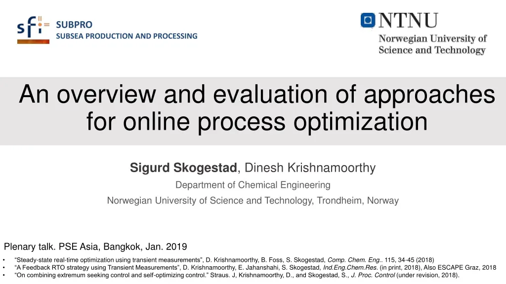
SUBPRO SUBSEA PRODUCTION AND PROCESSING. An overview and evaluation of approaches for online process optimization. Sigurd Skogestad , Dinesh Krishnamoorthy Department of Chemical Engineering Norwegian University of Science and Technology, Trondheim, Norway.

E N D
SUBPROSUBSEA PRODUCTION AND PROCESSING An overview and evaluation of approaches for online process optimization Sigurd Skogestad, Dinesh Krishnamoorthy Department of Chemical Engineering Norwegian Universityof Science and Technology, Trondheim, Norway Plenary talk. PSE Asia, Bangkok, Jan. 2019 • “Steady-state real-time optimization using transient measurements”, D. Krishnamoorthy, B. Foss, S. Skogestad, Comp. Chem. Eng.. 115, 34-45 (2018) • “A Feedback RTO strategy using Transient Measurements”, D. Krishnamoorthy, E. Jahanshahi, S. Skogestad, Ind.Eng.Chem.Res. (in print, 2018), Also ESCAPE Graz, 2018 • “On combining extremum seeking control and self-optimizing control.” Straus. J, Krishnamoorthy, D., and Skogestad, S., J. Proc. Control (under revision, 2018).
Trondheim Arctic circle
Outline • Introduction. • Why is traditional static RTO not used much? • Alternative approaches • Dynamic RTO • Hybrid RTO • Feedback RTO • Self-optimizing control • Extremum seeking control • Case studies • Gas lift, CSTR, Ammonia reactor
Hierarchical decision system Manager Process engineer min J (economics) hour Operator/RTO Focus ofthis talk Setpoint control (+ look after other variables) minute ”Advanced control”/MPC Stabilize + avoid drift second PID-control u = valves
Traditional static RTO • Most common in commercial RTO • Steady-state models • Two-step approach • “Data reconciliation”: • Steady-state detection • Update model parameters, disturbances (feed), constraints • Re-optimize to find new optimal steady state Data reconciliation D. E. Seborg, D. A. Mellichamp, T. F. Edgar, F. J. Doyle III, Process dynamics and control, John Wiley & Sons, 2010.
Traditional static RTO • Minimize static economic cost • Steady-state wait time – fundamental limiting factor • Process operates sub-optimally for long periods of time • Frequent disturbances • Long settling times
Why is traditionalstatic RTO not commonly used? In expected order of importance: «wait time» • It may seem that reasons 2, 4, and 5 suggest towards dynamic optimization. • However, except reason 4, static optimization may be close to the economic optimum, at a much lower computational cost. Cost of developing and updating the model (costly offline model update) Wrong value of model parameters and disturbances (slow online model update) Not robust, including computational issues Frequent grade changesmake steady-stateoptimization less relevant Dynamic limitations, including infeasibility due to (dynamic) constraint violation
Traditional static RTO: Long steady-state wait time • Challenges with steady-state detection • Erroneously accept transient data as stationary data • Large chunks of data discarded Câmara MM, Quelhas AD, Pinto JC. Performance Evaluation of Real Industrial RTO Systems. Processes. 2016, 4(4).
How to address steady-state wait time? • OBVIOUS: DYNAMIC RTO
Dynamic real-time optimization (DRTO) • Uses all (transient) data • Dynamic models • Dynamic optimization is computationally intensive • Closely related to economic MPC optimization
Economic MPC ~ Dynamic RTO MPC/PID • Centralized “All-in-one” optimizer • Higher sampling rates • Hierarchical layers with time scale separation • Lower sampling rates
Dynamic RTO has problems • Slow and not robust • Dynamic optimization is computationally expensive - even with today’s computing power • Numerical issues, convergence problems • Mixed-integer variables • Still an open problem, especially for dynamic problems
How to address problems with dynamic RTO? • Hybrid RTO • Feedback based RTO
Hybrid RTO Static RTO “Hybrid” RTO Dynamic RTO Dynamic Estimation + Static Optimization Krishnamoorthy, et al. (2018). Steady-State Real-time Optimization using Transient Measurements. Comput. & Chem. Eng., Vol 115, p.34-45.
Constraint: Max Gas capacity CASE STUDY: Gas lift Main objective: Max oil prod. MV1 MV2 Reservoir GOR = Gas/Oil ratio in feed (reservoir) Main disturbance (d): GOR variation
GOR estimation - using “data reconciliation” (traditional static RTO) Problem: Steady-statewait time for data reconciliation
Oil and gas rates SRTO = traditionalstatic RTO HRTO = hybrid RTO DRTO = dynamic RTO
Why is traditionalstatic RTO not commonly used? In expected order of importance: • It may seem that reasons 2, 4, and 5 suggest towards dynamic optimization. • However, except reason 4, static optimization may be close to the economic optimum, at a much lower computational cost. Cost of developing and updating the model (costly offline model update) Wrong value of model parameters and disturbances (slow online model update) Not robust, including computational issues Frequent grade changesmake steady-stateoptimization less relevant Dynamic limitations, including infeasibility due to (dynamic) constraint violation
Dynamic limitations – not a big issue with MPC-layer below MV2: Setpoint provided to tracking controller Actual MV move by setpoint tracking controller SRTO = traditionalstatic RTO HRTO = hybrid RTO DRTO = dynamic RTO
Discussion of Hybrid RTO • Addresses steady-state wait time issue • Need to maintain two models – Static and Dynamic • But not a big problem • But still have computational issues related to the static optimization
Advantage of steady-state optimization (SRTO & HRTO) • Computation time • Avoids causality issue: Allows optimization on decision variables other than the MVs • Simplifies the optimization • Slower time scale (choose slow varying variables as decision variables) • Example: Can specify directly maximum temperature and let controller find required input.
Alternative feedback-basedapproaches • New: Feedback RTO (faster computation) • Self-optimizing Control (SOC) (noonline modelupdateneeded) • Extremum-seekingcontrol (modelfree). Closelyrelated: • Evolutionary control (60’s) • Hill-climbing (Shinskey) • NCO-tracking
Feedback RTO: Replace steady-state optimization by feedback control Feedback RTO Hybrid RTO Krishnamoorthy, D., Jahanshahi, E. and Skogestad, S., 2018. A feedback real-time optimization strategy, Ind. Eng. Res. Chem (submitted).
CSTR case study • Economou, C. G.; Morari, M.; Palsson, B. O. Internal model control: Extension to nonlinear system. Industrial & Engineering Chemistry Process Design and Development 1986, 25, 403–411. • Ye, L.; Cao, Y.; Li, Y.; Song, Z. Approximating Necessary Conditions of Optimality as Controlled Variables. Industrial & Engineering Chemistry Research 2013, 52, 798–808.
Comparison of RTO approaches: MV SRTO = traditionalstatic RTO HRTO = hybrid RTO DRTO = dynamic RTO New method = Feedback RTO closer look t = 400 s, d1: IncreaseCAin t = 1400 s, d2: IncreaseCBin
Comparison of RTO approaches 342.3 257.1 248.1 247.1 2 3 1 4
Feedback RTO - Other case studies • Evaporator process1 • Gas lift wells2 • Ammonia reactor3 (14.45. Room 2) Krishnamoorthy, D., Jahanshahi, E. and Skogestad, S., Control of steady-state gradient for an Evaporator process, PSE Asia (Submitted 2019) Krishnamoorthy, D., Jahanshahi, E. and Skogestad, S., 2018. Gas-lift Optimization by Controlling Marginal Gas-Oil Ratio using Transient Measurements (in-Press), IFAC OOGP, Esbjerg, Denmark Bonnowitz, H., Straus, J., Krishnamoorthy, D., and Skogestad, S., 2018. Control of the Steady-State Gradient of an Ammonia Reactor usingTransientMeasurements, Computer aided chemical engineering, Vol.43, p.1111-1116 (ESCAPE 28)
Self-optimizing control Self-optimizing control is when we can achieve an acceptable loss with constant setpoint values for the controlled variables
Self-optimizing control (SOC) • Localapproximation: c = Hy. • Needdetailed steady-statemodel to find optimal H • Nullspace method • Exactlocalmethod • Must reoptimizefor eachexpecteddisturbance • Butcalculationsareoffline Challenges SOC: • Nonlinearity • Neednew SOC variables for eachactiveconstraint region • Similar to multiparametricoptimization and lookuptables
CSTR case study Feedback RTO («newmethod») Self-optimizing control Krishnamoorthy, D., Jahanshahi, E. and Skogestad, S., 2018. A feedback real-time optimization strategy, Ind. Eng. Res. Chem (submitted).
Why is traditionalstatic RTO not commonly used? Cost of developing and updating the model (costly offline model update) Wrong value of model parameters and disturbances (slow online model update) Not robust, including computational issues Frequent grade changesmake steady-stateoptimization less relevant Dynamic limitations, including infeasibility due to (dynamic) constraint violation
Challenges with structural uncertainty • Structural mismatch / unmodelled disturbances • Model simplification • Lack of knowledge • Modifier Adaptation • Model-free RTO approaches
Model-free methods • Extremum seeking control • NCO-tracking • Hill-climbing control
Serious challenges with model free methods • Needs cost measurement • Need additional perturbations • Steady-state limitation • Very slow convergence
Fix: ESC/RTO + Self-optimizing control • Self-optimization control is always complementary • Can combine with • Extremum-seeking control • Traditional Static RTO Straus. J, Krishnamoorthy, D., and Skogestad, S., 2018. On combining extremum seeking control and self-optimizing control. J. Proc. Control (under revision).
Whyis traditionalstatic RTO not commonly used?Somealternatives Cost of developing and updating the model (costly offline model update) Fix: modelfreemethods, like extremum-seeking 2. Wrong value of model parameters and disturbances (slow online model update) Fix: DRTO, HRTO, self-optimizing control (fastest) Not robust, including computational issues Fix: Feedback RTO, self-optimizing control Frequent grade changesmake steady-stateoptimization less relevant Fix: Dynamic RTO (DRTO) or EMPC Dynamic limitations, including infeasibility due to (dynamic) constraint violation Fix: MPC-layerbelow
Conclusion SUBPROSUBSEA PRODUCTION AND PROCESSING Ju Extremumseeking control/ Modifieradaptation Model free Extremelyslow (days) Ju,s Gradient estimator RTO: Detailedmodel (online) Real-time optimization (SRTO/DRTO/HRTO) Slow (hour) y cs c y Self-optimizing control (in MPC/PID layer) SOC: Detailedmodel (offline) Fast (minute) H u y Process Measurements d J • Thank you !
Commentsbasedondiscussionsafterwards • In practice: • Implementactiveconstraintsusingsupervisorylayer (selectors, SRC) or standrd MPC • Optimizeunconstrained DOFs usingextremumseeking control. Buteconomiccostcanusually not be measureddirectly, J = pF F + pQ Q – pP P • To obtaineconomiccostweneed a model to getflows F, P andc Q using data reconciliation.
Summary/Comparisononnext slide Red box = bad green box = good No box = neutral