Download

1 / 39
390 likes | 504 Vues
Health Risks of Exposure to Chemical Composition of Fine Particulate Air Pollution. Francesca Dominici Yeonseung Chung Michelle Bell Roger Peng Department of Biostatistics School of Public Health Harvard University. Chemical constituents. Size. Total mass. Groups. EC. OC. NH4 +.

E N D
Health Risks of Exposure to Chemical Composition of Fine Particulate Air Pollution Francesca Dominici Yeonseung Chung Michelle Bell Roger Peng Department of Biostatistics School of Public Health Harvard University
Chemical constituents Size Total mass Groups EC OC NH4 + SO4= PM2.5 PM10 Inorganic fraction of PM NO3- Si Ca PM10-2.5 Z Metals Al Ni Bell Dominici Ebisu Zeger Samet EHP 2007 Fe
New Scientific Questionsand Statistical Challenges What are the mechanisms of PM toxicity? • Size? • Chemical components? • Sources?
Three questions • Are day-to-day changes in the levels of the PM2.5 chemical components associated with day-to-day changes in admission rates? (short-term effects of PM2.5 components) • Multi-site time series studies of PM components • Are the short-term effects of PM2.5 total mass on admission rates modified by long-term averages of PM2.5 chemical components? • Multi-site time series studies of PM total mass and second stage regression on PM components • Are the long-term effects of PM2.5 total mass on mortality modified by long-term averages of PM2.5 components? • Spatially varying coefficient models
The National Medicare Cohort Study, 1999-2009 (MCAPS) • Medicare data include: • Billing claims for everyone over 65 enrolled in Medicare (~48 million people), • date of service • disease (ICD 9) • age, gender, and race • place of residence (zip code) • Approximately 204 counties linked to the PM2.5 monitoring network
MCAPS study population: 204 counties with populations larger than 200,000 (11.5 million people)
Daily time series of hospitalization rates and PM2.5 levels in Los Angeles county (1999-2005)
Exposure data: Chemical composition data on PM2.5 from the STN network • Constructed a database of time series data for 52 PM2.5 chemical constituents from over 250 STN monitors for 2000 to 2008 • Identified a subset of PM2.5 components that substantially contribute and/or co-vary with daily PM2.5 concentrations • Constructed a database that links by zip code the chemical composition data to human health data Bell et al EHP 2007
Chemical composition data on PM2.5 • Only seven of the 52 components contributed 1% or more to total mass for yearly or seasonal averages • OCM • Sulfate • Nitrate • EC • Silicon • Sodium Ion • Ammonium
Multi-site time series data • Semi-Parametric Regression for time series data • Hierarchical Models for combining health risks across locations • Model Uncertainty in effect estimation
JASA 2004 • Confounders: • weather variables • seasonality
Smooth part Everson and Morris, JRSSB 2000 Dominici Samet Zeger JRSSA 2000 R package for TLNISE, released on March 26 2008 by Roger Peng
Assessing the sensitivity of the results to model assumptions • Sensitivity of the exposure effect estimate to: • the number of degrees of freedom in the smooth functions of time to adjust for seasonality • the degree of flexibility in the adjustment for weather variables • other potential confounders (e.g other pollutants)
PM2.5 and Admissions PM10-2.5 and Admissions Dominici et al JAMA 2006 Peng et al JAMA 2008 US EPA PM Fact Sheet 2006: To better protect public health EPA issued the Agency most protective suite of national air quality standards for particle pollution ever
National average estimates and 95% posterior intervals for the percent increase in hospital admissions for cardiovascular diseases per 1 IQR increase in each of the seven PM2.5 components, 119 U.S. counties, 2000--2006. Peng et al submitted Peng et al 2008, EHP
Do the PM2.5 chemical constituents modify the short-term effects of PM2.5 on mortality and morbidity?% increase in CVD-PM2.5 risk per IQR increase in the fraction of PM2.5 total mass for each component. Statistically significant associations are shown in bold 101 US counties 1999-2005 Bell et al AJRCCM 2009
Average PM2.5 levels for the period 2000 to 2006 for 518 monitors in the East US
Bayesian Spatially Varying Coefficient Models for estimating spatially varying long term effects of PM2.5 (Stage I) Mortality counts in zip codes “close” to monitor “i” average PM2.5 • “i” is the monitor • “j” is the month • “xij” is the average PM2.5 over the 12 previous months
Bayesian Spatially Varying Coefficient Models for estimating spatially varying long term effects of PM2.5 (Stage II) Long-term average of log relative proportion of kth component Spatial Coordinate of ith location Investigating whether PM2.5 chemical components explain the spatial variability in mortality risks
Missing data challenge • The monitoring network that provides the chemical composition (STN) data is sparser than and does not exactly match with the PM2.5 monitoring stations. • For 241 monitors we have both PM2.5 and composition data • For 277 monitors we have PM2.5 but composition is missing • For 10 monitors we have composition data but PM2.5 is missing. 518 241 251 sparser than Composition data available All spatial units in our analysis
Analysis options Option 1. Using only 241 locations where the chemical composition data are available Option 2. Using all 518 locations with an imputation procedure for missing composition data incorporated in the model
Option 1 : using 241 locations Table 1. Posterior median for each parameter with 95% credible intervals Posterior median for slope: Posterior median for slope:
Option 2 : using 518 locationsConstructing a prior for ZMiss • We propose a prior for the missing composition data and incorporate an imputation procedure in the MCMC iterations. • We denote the component levels for 3 different locations as • We assume the component levels for observed + extra locations come from a multivariate Gaussian spatial process as • We obtain posterior estimates for using a spBayes R package (Finley et al., 2010). : # of missing locations ZMiss 277 : # of observed locations 518 ZObs : # of extra locations ZExtra 10 241 251
Option 2 : using 518 locationsConstructing a prior for ZMiss • We propose a prior for the missing composition data and incorporate an imputation procedure in the MCMC iterations. • Using , we specify a multivariate Gaussian process for the component levels for missing+observed locations. • We derive the conditional distribution for ZMiss given Zobs • Because the component levels cannot be negative, we use a truncated version of the above multivariate Gaussian process as a prior for ZMiss
Option 2 : using 518 locations • The hierarchical structure of our full Bayes model is Likelihood Prior for fixed effects Prior for ZMiss Prior for spatially correlated random effects
OCobs OCobs+pred SO4obs SO4obs+pred Siobs Siobs+pred ECobs ECobs+Pred NO3obs NO3obs+pred Sodobs Sodobs+pred
Effect modification of the long term effects of PM2.5 on mortality by PM2.5 composition (Using 241 locations) (Using 518 locations) Effect on Intercept Effect on Slope Dot is posterior median and line indicates 95% credible interval.
Summary • We used three study designs to address three related epidemiological questions on the toxicity of PM2.5 • We implemented MCMC algorithms for very large data sets
Summary We found that: • PM10-2.5, (e.g. crustal materials) lead to smaller health risks than PM2.5 (e.g.combustion-related constituents) • EC and OCM, which are generated typically from vehicle emissions, diesel, and wood burning, lead to the largest risk of emergency hospital admissions for cardiovascular and respiratory diseases compared to the other PM2.5 chemical constituents Combustion sources Crustal materials
Sub-region analysis Table 1. Posterior median for other parameters with 95% credible intervals
Option 2 : using 518 locations • Our model can be written as Main effects interactions • The likelihood function is
References • Chung Y, Dominici F, Bell M Bayesian Spatially Varying Coefficients Models of Long term effects of PM2.5 and PM2.5 composition (in progress) • Papers in blue have been presented in these slides
Option 2 : using 518 locationsConstructing a prior for ZMiss • We denote the component levels for 3 different locations as • We assume that the component levels for observed + extra locations come from a multivariate Gaussian spatial process as • We obtain posterior estimates for using a spBayes R package (Finley et al., 2010). ZMiss 277 ZObs 518 ZExtra 10 241 251
Constructing a prior for ZMiss • Using , we specify a multivariate Gaussian process for the component levels for missing+observed locations. • We derive the conditional distribution for ZMiss given Zobs
Option 2 : using 518 locations • We place a prior for ZMiss and incorporate an imputation procedure in the MCMC iterations. The prior can be obtained from a multivariate spatial process defined for ZMiss, Zobs, ZExtra (Next Slide). We obtain posterior estimates for using a spBayes R package (Finley et al., 2010).