Download
1 / 27
270 likes | 432 Vues
More Regression. What else?. General Outline. Dealing with categorical data Dummy coding Effects coding Different approaches to MR Standard Sequential Stepwise Model comparison Moderators and Mediators. Categorical variables in regression. Dummy coding 0s and 1s

E N D
More Regression What else?
General Outline • Dealing with categorical data • Dummy coding • Effects coding • Different approaches to MR • Standard • Sequential • Stepwise • Model comparison • Moderators and Mediators
Categorical variables in regression • Dummy coding • 0s and 1s • p-1 predictors will go into the regression equation leaving out one reference category (e.g. control) • Note that with only 2 categories the common 0-1 classification is sufficient to use directly in MR • Coefficients will be interpreted as change with respect to the reference variable (the one with all zeros)
Dummy coding • In general, the coefficients are the distances from the dummy values to the reference value, controlling for other variables in the equation • Perhaps the easier way to interpret it is not in terms of actual change in Y as we do in typical regression (though that’s what we’re doing), but how we do in Anova with regard to mean differences • The b coefficient is how far the group mean is from the reference group mean, whose mean can be seen in the output as the constant • The difference in coefficients is the difference between means • If only two categories, the b represents the difference in means
Effects coding • Makes comparisons in relation to the grand mean of all subgroups • Reference category is coded as -1 for all predictor dummy variables • Still k-1 predictors for k groups • Given this effect coding, a b of -1.5 for the dummy “Experimental Group 2" means that the expected value on the DV for the Experimental (i.e. its mean) is 1.5 less than the mean for all subgroups • Dummy coding interprets b for the dummy category relative to the reference group (the left-out category), effects coding interprets it relative to the entire set of groups • Perhaps more interpretable when no specific control group for reference
Contrast coding • Test for specific group differences and trends • Coding scheme the same as done in Anova • http://www.ats.ucla.edu/stat/sas/webbooks/reg/chapter5/sasreg5.htm
Methods of MR • Sequential/Hierarchical • Stepwise
Sequential* (hierarchical) regression • Researcher specifies some order of entry based on theoretical considerations • They might start with the most important predictor(s) to see what they do on their own before those of lesser theoretical interest are added • Otherwise, might start with those of lesser interest, and see what they add to the equation (in terms of R2) • There isn’t any real issue here, except that you can get the same sort of info by examining the squared semi-partial correlations with the ‘all in’ approach
Comparison of Standard vs. Sequential • Standard at top, 3 different orderings follow • Note that no matter how you start you end up the same once all the variables are in.
Take the squared semi-partials from the previous slide (appropriate model) and add them in to get your new R2 • For example from the first ordering, to get from E to E+B i take the part correlation for B (.790) square it, and add to .063 (the R2 with E only) to get my new R2 of .688
Sequential regression • The difference between standard and sequential regression is primarily one of description of results, not method • In standard we are considering each variable as if it had been entered last in an sequential regression, partialling out the effects of other variables • Akin to ‘Type III’ sums of squares in Anova setting • Sequential may provide a better description of your theory, and allow you to do sets at a time rather easily, but the info is technically there to do so in a standard regression
Stepwise (statistical) methods • Statistical methods allow one to come up with a ‘best’ set of predictors from a given number • Backward • Forward • “Stepwise” • All possible subsets
Stepwise • Backward • All in • Remove least ‘significant’ contributor • Rerun, do the same until all left are significantly contributing • Forward • Start with predictor with largest correlation (validity) with DV • Add in the next predictor that results in e.g. greatest increase in R2 • The third will be added with the first two staying in • Continue until no significant change in model results from the addition of another variable
Stepwise • “Stepwise” • Forward and backward are both stepwise procedures • “Stepwise” specifically refers to the forward selection process, but if upon retest of a new model a variable previously significant is no longer so, it is removed • All subsets • Just find the best group of variables out of many based on some criterion, or just choose from the results which one you like
Problems with stepwise methods • Capitalization on chance • Results are less generalizable and may only hold for your particular data • SPSS, i.e. the statistical program, is dictating your ideas • “Never let a computer select predictors mechanically. The computer does not know your research questions nor the literature upon which they rest. It cannot distinguish predictors of direct substantive interest from those whose effects you want to control.” (Singer & Willett)
Problems with stepwise methods • Frank Harrell (noted stats guy) • It yields R-squared values that are badly biased high. • The F and chi-squared tests quoted next to each variable on the printout do not have the claimed distribution. • The method yields confidence intervals for effects and predicted values that are falsely narrow (See Altman and Anderson, Statistics in Medicine). • It yields P-values that do not have the proper meaning and the proper correction for them is a very difficult problem. • It gives biased regression coefficients that need shrinkage (the coefficients for remaining variables are too large; see Tibshirani, 1996). • It has severe problems in the presence of collinearity. • It is based on methods (e.g., F tests for nested models) that were intended to be used to test prespecified hypotheses. • Increasing the sample size doesn't help very much (see Derksen and Keselman). • It allows us to not think about the problem.
More • Stepwise methods will not necessarily produce the best model if there are redundant predictors (common problem). • Models identified by stepwise methods have an inflated risk of capitalizing on chance features of the data. They often fail when applied to new datasets. They are rarely tested in this way. • Since the interpretation of coefficients in a model depends on the other terms included, “it seems unwise to let an automatic algorithm determine the questions we do and do not ask about our data”. • “It is our experience and strong belief that better models and a better understanding of one’s data result from focused data analysis, guided by substantive theory.” • Judd and McClelland, Data Analysis: A Model Comparison Approach
Model comparison • Multiple regression allows us to pit one hypothesis/theory vs. another • Is one set of predictors better at predicting a DV than another set? • Can get a z-score for the difference between two R2 • Note however, that R2s that aren’t that far off could change to nonsig difference or even flip flop upon a new sample • Always remember that effect sizes, like p-values are variable from sample to sample
Model comparison • Interpret as you normally would a z-score • Multiple R for set of predictors A. Same would be done for other set of predictors B. rab would be the correlation b/t two opposing predictors, or the canonical correlation between sets of predictors
Model comparison • Other statistics allow for a comparison as well • Fit statistics such as AIC or BIC that you typically see in path analysis or SEM might be a better way to compare models
Moderators and Mediators • Moderators and mediators are often a focus of investigation in MR • First thing to do is keep them straight • Moderators • Same thing as an interaction in ANOVA • Mediators • With the mediator we have a somewhat different relationship between the predictor variables, such that one variable in effect accounts for the relationship between an independent and dependent variable. • As you can see, these are different relationships and will require different tests
Moderators • In typical analysis of variance, interactions are part of the output by default. • In multiple regression, interactions are not as often looked at (though probably should be more), and usually must be specified. • As with anova (GLM), the interaction term must be added to the equation as the product of the IVs in question • Continuous variables should be centered • Transform the variable to one in which the mean is subtracted from each response (alternatively one could use z-scores). • This will primarily deal with the collinearity issue we’d have with the other IVs correlating with the new interaction term • In addition, categorical variables must be transformed using dummy or effects coding. • To best understand the nature of the moderating relationship, one can look at the relationship between one IV at particular (fixed) levels of the other IV
Variable A Criterion Moderator B C Variable X Moderator Moderators • Also, we’re not just limited to 2-way interactions • One would follow the same procedure as before for e.g. a 3-way, and we’d have the same number and kind of interactions as we would in Anova
Mediators • Mediator variables account for the relationship between a predictor and the dependent variable • Theoretically, one variable causes another variable which causes another • In other words, by considering a mediator variable, an IV no longer has a relationship with the DV (or more liberally, just decreases)
Mediators • Testing for mediation • To test for mediators, one can begin by estimating three regression equations • (1) The mediator predicted by the independent variable • (2) The dependent variable predicted by the independent variable • (3) The dependent variable predicted by the mediator and independent variable. • To begin with, we must have significant relationships found for the equations (1) and (2). • If the effect of the IV on the DV decreases dramatically when the mediator is present (e.g., its effect becomes nonsignificant), then the mediator may be accounting for the effects of the independent variable in question. • Overall power for equation (3) is diminished due to the correlation between the independent variable and mediator, and so rigid adherence to the p-value may not tell the whole story. • Also look at the size of the coefficients, namely, if the coefficient for the independent variable diminishes noticeably with the addition of the mediator to the equation.
Mediators • Sobel test for mediation • Calculate a, which equals the unstandardized coefficient of the IV when predicting the DV by itself, and its standard error sa. From equation (3) take the unstandardized coefficient b for the mediator and its standard error sb. • To obtain the statistic, input those calculations in the following variant of the Sobel’s original formula: • Test of the null hypothesis that the mediated effect (i.e. a*b or c-c’, where c’ = the relationship after controlling for the mediator) equals zero in the population
Moderators and Mediators • Mediators and moderators can be used in the same analysis* • More complex designs are often analyzed with path analysis or SEM