Download

1 / 49
500 likes | 677 Vues
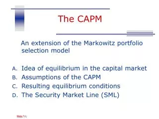
CHAPTER 8 CAPM Models. 8.1 THE CAPM MODEL. Capital Asset Pricing Model. Equilibrium model that underlies all modern financial theory Provide benchmark rate of return for evaluating possible investments Make an educated guess as to the expected return

E N D
Capital Asset Pricing Model • Equilibrium model that underlies all modern financial theory • Provide benchmark rate of return for evaluating possible investments • Make an educated guess as to the expected return • Derived using principles of diversification with simplified assumptions • 1964, Markowitz, 1965,Sharpe, 1966,Lintner and Mossin are researchers credited with its development
Assumptions • Perfect competition assumption, Individual investors are price takers • Single-period investment horizon • Investments are limited to traded financial assets, may borrow or lend any amount at a fixed risk-free rate • No taxes nor transaction costs
Assumptions (cont.) • Information is costless and available to all investors • Investors are rational mean-variance optimizers • Homogeneous expectations, analyze securities in the same way and share the same economic view of the world • same input list to feed into the Markowitz model • Same E(r), covariance matrix, same efficient frontier and unique optimal risky portfolio
Resulting Equilibrium Conditions • All investors will hold the same portfolio for risky assets –market portfolio (M) • Market portfolio contains all securities and the proportion of each security is its market value as a percentage of total market value • Capital market line (CML) is the best attainable CAL
Resulting Equilibrium Conditions Risk premium on the market portfolio depends on the average risk aversion of all market participants (explained in P9)
Resulting Equilibrium Conditions Risk premium on an individual security will be proportional to the risk premium on M and beta coefficient of the security relative to M
Why holding the market portfolio Value of the aggregate risky portfolio will equal the entire wealth of the economy Use identical Markowitz analysis, same universe of securities, same time horizon, same input list, must arrive at the same composition of the optimal risky portfolio When all investors have same risky portfolio, it must be M.
Risk Premium of the Market Portfolio The market portfolio is the optimal risky portfolio (tangency portfolio) To decide how much in risky portfolio, how much in risk-free asset? Net borrowing and lending among all investors must be zero, y=1
Expected Returns On Individual Securities To measure the GM’s contribution to the risk of the market portfolio (the manner: sum of the contributions of each stock equals the total variance) variance of the portfolio: sum over all the elements of the covariance matrix The contribution of GM to the market portfolio variance is the sum of the GM covariance row
Expected Returns On Individual Securities demonstration
Expected Returns On Individual Securities Contribution of GM to the risk premium of the market portfolio The reward-to-risk ratio for GM
Expected Returns On Individual Securities M is the tangency portfolio, the market price of risk: When equilibrium, all investors have same reward-to-risk ratio
Expected Returns –Beta relationship Beta measures the contribution of GM to the market variance as a fraction of the total variance of the market portfolio
Expected Returns –Beta relationship CAPM holds for the overall portfolio
Security Market Line • Beta measures stock’s contribution to variance of market portfolio, required risk premium to be a function of beta. • Security Market Line: • The expected return-beta relationship be portrayed • Individual asset risk (or portfolio) premium as a function of asset risk, using beta as risk measurement • Capital Market Line: • The expected return-std deviation relationship • Risk premiums of efficient portfolios (composed of market and risk-free asset) as a function of portfolio standard deviation.
Security Market Line • SML provide benchmark for evaluation • Risk measured as Beta, SML provide the required rate of return • Fairly priced assets plot exactly on SML • Given the assumptions, all securities must lie on the SML in market equilibrium • Under-priced plot above, over-priced below • Alpha • difference between the fair and actually expected rate of return on a stock • Useful in capital budgeting decisions • Required rate of return that the project need to yield based on its beta (IRR)
Security Market Line • SML provide a benchmark for the evaluation of investment performance • provide the required rate of return • Fairly priced assets plot exactly on the SML • Under-priced plot above, over-priced below • Alpha • difference between the fair and actually expected rate of return on a stock
Actual returns versus expected return • CAPM: expected return, ex ante • Not feasible to construct M, difficult in testing variance efficiency of the CAPM market portfolio • CAPM implies relationships among expected returns, to calculate the reward-to-volatility ratio, but no way to observe the expectations directly • Index model: Actual (realized) return, ex post
Index model and CAPM Index model: Actual (realized) return, ex post Index model beta coefficient is the same beta in CAPM.
Index model and the expected return-beta relationship In CAPM: mean excess return of stock i relative to mean excess return of market portfolio If the M in index model represent the true market portfolio, take expectation ofindex model CAPM predict Alpha=0. Alpha of a stock is its expected return in excess of (or below) the fair expected return as predicted by the CAPM
Index model and the expected return-beta relationship Comparison of CAPM and Index model CAPM predicts that alpha should be zero for all assets, if the stock is fairly priced its alpha must be zero (expected return) Index model representation of the CAPM holds that the realized value of alpha should average out to zero for a sample of historical observed returns (if estimate the index model for several firms for a sample period) JOF 1995, distribution of alpha is roughly bell shaped, mean is slightly negative but statistically indistinguishable from zero Not appear that mutual funds outperform the market index
Figure 9.4 Estimates of Individual Mutual Fund Alphas, 1972-1991
Index model and the expected return-beta relationship Market model- applicable variation of index model Return surprise of any security is proportional to the return surprise of the market plus a firm-specific surprise If CAPM is valid, market model is identical to the index model
The CAPM and Reality Role of CAPM in real-life investment Notion that all alpha can be zero is feasible in principle, but not expected to emerge in real markets (Grossman and Stiglitz, 1981) such an equilibrium may be one that the real economy can approach, but not necessarily reach actions of security analysts are forces that drive security prices to proper levels (alpha=zero) In the absence of security analysis , one should take security alphas as zero, obtain the best investment portfolio on the assumption that all alpha values are zero
The CAPM and Reality Is the CAPM testable Proxies must be used for the market portfolio, unobservable CAPM fails the test, data reject the hypothesis that alpha are uniformly zero Result of a failure of data, validity of the market proxy or statistical method CAPM is still considered the best available description of security pricing and is widely accepted
Econometrics and the Expected Return-Beta Relationship • It is important to consider the econometric technique used for the model estimated • Statistical bias is easily introduced • Miller and Scholes paper demonstrated how econometric problems could lead one to reject the CAPM even if it were perfectly valid
EXTENSIONS OF CAPM • Two kinds of extension to the simple version of CAPM • Relax the assumptions • Consider more risk factors other than the uncertain value of the securities, such as unexpected changes in relative prices of consumer goods.
Extensions of the CAPM Assumption: all risky assets are traded Human capital and privately held corporations Consideration of labor income and non-traded assets
Extensions of the CAPM Assumption: single-period Merton 1992, individuals optimize a lifetime consumption, continually adapt consumption. Sources of risk, changes of parameters describing investment opportunities, such as future risk-free rates , risk of market portfolio Prices of the consumption goods that can be purchased with any amount of wealth Merton’s Multi-period Model and hedge portfolios Incorporation of the effects of changes in the real rate of interest and inflation
Extensions of the CAPM Continued • A consumption-based CAPM • Models by Rubinstein, Lucas, and Breeden • Investor must allocate current wealth between today’s consumption and investment for the future • C: consumption-tracking portfolio
Liquidity and the CAPM Trading is of importance to investors (heterogeneous expectations), trading costs Liquidity: ease and speed with which it can be sold at fair market value Cost of engaging in a transaction, bid-ask spread Price impact, adverse movement in price when attempt to execute a larger trade Immediacy, ability to sell the asset quickly without reverting to fire-sale prices Illiquidity can be measured in part by the discount from fair market value a seller must accept if the asset is to be sold quickly Research supports a premium for illiquidity. Amihud and Mendelson (1986)
CAPM and Liquidity Illiquidity premium Begin with Ignorance of systematic risk, T-bill N type of investors (n periods), investment horizon
CAPM and Liquidity Stock L and stock I prices must fall, causing their return to rise Suppose each gross return is higher by some fraction of liquidation cost
CAPM and Liquidity • When h increases, less impact. As horizon become large, per-period impact of the transaction cost approaches zero
CAPM and Liquidity Equilibrium illiquidity premium for marginal investor with horizon , net return( I=L) Expected return on stock I
CAPM and Liquidity Expected return of stock L Illiquidity premium of stock I versus stock L
CAPM and Liquidity for marginal investor with horizon , net return( T-bill=L) Liquidity premium of stock L
CAPM and Liquidity • Inventory management problem, bid-ask spread may be viewed as compensation for bearing the price risk involved in holding an inventory of securities • Component of the spread due to asymmetric information • Traders who post offers to buy or sell at limit prices need to be worried about being picked off by better-informed traders • Trading for tow reasons: • non-informational motives, liquidity traders, noise trades, not motivated by private information, dealers earn profit from bid-ask spread • Information traders, motivated by private information known only to the seller or buyer, impose a cost on both dealers and other investors • Any traders posting a limit order is at risk from information traders, response is to widen spread to compensate for potential losses from trading with information traders
CAPM and Liquidity When consider common systematic risk factors, illiquidity premium is additive to the risk premium or the usual CAPM is expected cost of illiquidity, beta is liquidity betas
Three Elements of Liquidity Sensitivity of security’s illiquidity to market illiquidity: Sensitivity of stock’s return to market illiquidity: Sensitivity of the security illiquidity to the market rate of return: