Download
1 / 41
450 likes | 698 Vues
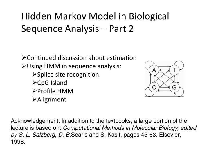
Hidden Markov Model in Biological Sequence Analysis – Part 2. Continued discussion about estimation Using HMM in sequence analysis: Splice site recognition CpG Island Profile HMM Alignment.

E N D
Hidden Markov Model in Biological Sequence Analysis – Part 2 • Continued discussion about estimation • Using HMM in sequence analysis: • Splice site recognition • CpG Island • Profile HMM • Alignment Acknowledgement: In addition to the textbooks, a large portion of the lecture is based on: Computational Methods in Molecular Biology, edited by S. L. Salzberg, D. B.Searls and S. Kasif, pages 45-63. Elsevier, 1998.
HMM p11 b1(A1) A1 A2 E1 E2 b1(A2) p12 p21 b2(A1) Initiation b2(A2) p22 initial distribution transition probabilities emission probabilities
Hidden Markov Model Common questions: How to efficiently calculate emissions: How to find the most likely hidden state: How to find the most likely parameters: Notations: Let denote the hidden state sequence; Let denote the observed emission sequence; Let denote the emission up to time t.
Reminders Calculating emissions probabilities: Emissions up to step t chain at state i at step t
Reminders Calculating posterior probability of hidden state: Emissions after step t chain at state i at step t
The Viterbi Algorithm To find: So, to maximize the conditional probability, we can simply maximize the joint probability. Define:
The Viterbi Algorithm Then our goal becomes: Compare this to dynamic programming pairwise sequence alignment: At every step, we aim at the maximum The maximum depends on the last step At the end, we want the maximum and the trace So, this problem is also solved by dynamic programming.
The Viterbi Algorithm Time: 1 2 3 States: E1 0.5*0.5 0.15 0.0675 E2 0.5*0.75 0.05625 0.01125 The calculation is from left border to right border, while in the sequence alignment, it is from upper-left corner to the right and lower borders. Again, why is this efficient calculation possible? The short memory of the Markov Chain!
The Estimation of parameters When the topology of an HMM is known, how do we find the initial distribution, the transition probabilities and the emission probabilities, from a set of emitted sequences? Difficulties: Usually the number of parameters is not small. Even the simple chain in our example has 5 parameters. Normally the landscape of the likelihood function is bumpy. Finding the global optimum is hard.
Basic idea There are three pieces: λ, O, and Q. O is observed. We can iterate between λ and Q. When λ is fixed, we can do one of two things: (1) find the best Q given O or (2) integrate out Q When Q is fixed, we can estimate λ using frequencies.
The Viterbi training Start with some initial parameters (2) Find the most likely paths using the Viterbi algorithm. (3) Re-estimate the parameters. On next page. (4) Iterate until the most likely paths don’t change.
The Viterbi training Estimating the parameters. Transition probabilities: Emission probabilities: Initial probabilities: need multiple training sequences.
Baum-Welch algorithm • The Baum-Welch is a special case of the EM algorithm. • The Viterbi training is equivalent to an simplified version of the EM algorithm, replacing the expectation with the most likely classification. • General flow: (1) Start with some initial parameters (2) Given these parameters, P(Q|O) is known for every Q. This is done effectively by calculating the forward and the backward variables. (3) Take expectations to obtain new parameter estimates. (4) Iterate (2) and (3) until convergence.
Baum-Welch algorithm Reminder: Estimation of emission probabilities:
Baum-Welch algorithm time t t+1 State i State j Emission Ot Ot+1
Baum-Welch algorithm Estimation of transition probabilities: Estimation of initial distribution:
Baum-Welch algorithm • Comments: • We don’t actually calculate P(Q|O). Rather, the necessary information pertaining to all the thousands of P(Q|O) is summarized in the forward- and backward- variables. • When the chain runs long, logarithm need to be used for numerical stability. • In applications, the emission is often continuous. A distribution need to be assumed, and the density used for emission probabilities. • The Baum-Welch is a special case of the EM algorithm. • The Viterbi training is equivalent to an simplified version of the EM algorithm, replacing the expectation with the most likely classification.
Common questions in HMM-based sequence analysis • HMM is very versatile in terms of coding sequence properties by model structures. • Given a sequence profile (HMM with parameters known), find the most likely hidden state path from a sequence. • A harder question: • Given a bunch of (aligned) training sequence segments, • - find the most plausible HMM structure • -- train the parameters of the HMM.
Splice site recognition E: exon I: intron 5: 5’splice site Nature Biotech. 22(10): 1315
CpG Island In the four character DNA book, the appearance of “CG” is rare, due to some issues related to the probability of mutations. However, there are regions where “CG” is more frequent. And such regions are mostly associated with genes. (Remember, only 5% of the DNA sequence are genes. ) ……GTATTTCGAAGAAT……
CpG Island A+ C+ G+ T+ G- T- A- C- Within the “+” and “-” groups, the transition probabilities are close to shown in the table. A small probability is left for between “+” and “-” transitions.
CpG Island Transition probabilities are summarized from known CpG islands. To identify CpG island from new sequences: Using the most likely path: run the Viterbi algorithm. When the chain passes through any of the four “+” states, call it an island Using the posterior decoding: run the forward- and backward- algorithm. Obtain the posterior probabilities of each letter being in a CpG island.
Profile HMM --- a simple case Motif: functional short sequence that tends to be conserved.
Profile HMM --- a simple case For (1) accounting for sequence length, (2) computational stability, Log odds ratios are preferred.
Profile HMM --- the general model Deletion Insertion
Profile HMM --- the general model Avoid over-fitting with limited number of observed sequences. Add pseudocounts proportional to the observed frequencies of the amino acids. And add pseudocounts to transitions.
Profile HMM --- searching with profile HMM Given a profile HMM, how to find if a short sequence is such a motif? Use the Viterbi algorithm to find the best fit and the log odds ratio:
Multiple sequence alignment (1) From a known family of highly related sequences, find the most conserved segments which have functional and/or structural implications. Pandit et al. In Silico Biology 4, 0047
Multiple sequence alignment (2) From a known family of sequences that are related only by very small motifs (that contribute to the function), find the real motif from vast amounts of junk. This is a harder problem that draws statisticians. Science262, 208-214.
Heuristic methods for global alignment • Scoring: Sum of Pairs (SP score) • Assume columns of the alignment is independent from each other • For each column, the score is the sum of the scores between all possible pairs • For the overall alignment, the score is the sum of the column scores
Heuristic methods for global alignment Multi-dimensional dynamic programming: 2N-1choices at each step. Impractical with more than a few sequences.
Heuristic methods for global alignment Progressive alignment: when exhaustive search is hard, go stepwise.
Heuristic methods for global alignment MSA: reducing multi-dimensional dynamic programming search space based on fast methods like progressive alignment.
Heuristic methods for global alignment CLUSTALW: profile alignment rather than purely pairwise Key improvement: Once an aligned group of sequences is established, position-specific information from the group is used to align a new sequence to it.
Heuristic methods for global alignment Alignment by profile HMM training. We have studied the scoring system by known HMM. The difficulty here is to train the HMM from unaligned sequences. Baum-Welch and Viterbi can be trapped by local optima. Stochastic methods like simulated annealing can help.
Heuristic methods for global alignment Alignment by profile HMM training. For global alignment, the number of matching states is ~mean(sequence length). The motif discovery we will talk about also utilizes the HMM in essence. The difference is in motif models, only a very small number of (5~20) matching states is expected. The vast amount of data is generated from a relatively simple background chain.
Modeling genes with HMM Genes account for only 5% of the human genome. Within each gene, there are exons (that code for protein sequence) and introns (that are skipped during transcription). Characteristics of the exons, introns and the borders between them allow people to identify putative genes from long DNA sequences. HMM is a model that can incorporate such characteristics.