Download
1 / 32
320 likes | 451 Vues
CBRFC Workshop SLC , 21mar11. Long-Range Forecasting. Klaus Wolter University of Colorado, CIRES & NOAA-ESRL PSD 1, Climate Analysis Branch klaus.wolter@ noaa.gov. • ENSO signal in Western U.S. • What is different this year?

E N D
CBRFC Workshop SLC, 21mar11 Long-Range Forecasting Klaus Wolter University of Colorado, CIRES & NOAA-ESRL PSD 1, Climate Analysis Branch klaus.wolter@noaa.gov •ENSO signal in Western U.S. •What is different this year? •One decade of real-time statistical climate predictions (‘SWcasts’) • Lees Ferry Water Year streamflow forecasts • Next steps
Assessment of current ‘state of the art’ climate forecasting • ‘Workhorse’ tools are mostly statistical, but ‘get no respect’; this includes current CPC toolbox that uses four different statistical tools and one dynamical tool (that has to match statistical tools to be taken seriously); ENSO came into play in late ‘80s, and ‘OCN’ in mid-90s; while forecasts are made out to 15 months, they rarely utilize ENSO information beyond ~ six months; OCN could be used to longer time scales, but has signal mainly in temperatures (surprisingly weak in last few years); • Coupled climate models (CFS) have come a long way, but are (IMHO) not quite ready yet to replace statistical tools; • +++++++++++++++++++++++++++++++++++++++++++++++++++++++++++++ • My own statistical efforts are essentially a race against time to see how much more signal can be extracted from data before climate stationarity assumption goes out the ‘Greenhouse’ window… • Better ENSO monitoring with MEI than with Niño 3.4 SST; • Higher signal-to-noise ratio withimproved climate divisions (predictands); • Careful expansion of predictors outside ENSO.
How should we monitor ENSO? The Multivariate ENSO Index was developed to summarize major components of ENSO system in a single index, using the first unrotated Principal Component of six atmosphere-ocean variables: SLP, zonal& meridionalsurface winds, SST, air temperature, and cloudiness. http://www.esrl.noaa.gov/psd/people/klaus.wolter/MEI/
How should we monitor ENSO? In order to allow for the combination of six atmosphere-ocean variables, each field is normalized to have standardized units. The resulting combined MEI time series has varied from about -2 sigma (standard deviations) to +3, while the long-term mean value is zero. This index correlates highest with other ENSO indices during boreal winter (≥0.90 with Niño 3.4), but drops off during spring and summer (~0.7). The MEI is the only ENSO index that is normalized for the season it monitors (Niño 3.4 standard deviations vary by a factor of two thru the annual cycle). http://www.esrl.noaa.gov/psd/people/klaus.wolter/MEI/
What are typical ENSO impacts in Western U.S.? SEP-NOV MEI vs. seasonal precipitation: Upper Colorado basin tends to be dry with La Niña in fall and spring, but WET in winter, especially at higher elevations of northern Colorado! DEC-FEB MAR-MAY ENSO signal is not weak in Upper Colorado, just spatially and seasonally variable!
La Niña springs Individual spring months show typically dry behavior in March (top left), May (middle), and June (bottom right) in the wake of a La Niña winter, while April (top right) is another story, most recently in 1999.
U.S. Climate Divisions This is a map of 344 climate divisions currently in use over the U.S. Note the changing size as one goes from east to west, as well as from one state to another. CPC originally used 102 mega or forecast divisions in their forecasts. The divisions in the West closely correspond to NCDC climate divisions. Most of their statistical tools were developed using these data. <this is like looking through coke bottles>
Interior Southwest experimental climate divisions Improved seasonal PREDICTANDS based on COOP and SNOTEL station data - first generation effort, in use since 2000. Amount of color in each station symbol proportional to locally explained variance via divisional time series.
New Climate Divisions for Colorado River Basin Some of the remaining issues: What to do with undersampled regions (American Indian nations, SW Wyoming)? How to match climate divisions with HUCs? Can we trust the pre-SNOTEL era when COOP records are the only available data? <Some regions have much better historical record (~100 vs. 50 years) than others.>
An empirical effort to improve climate forecasts Recent practice at CPC: ENSO + OCN (trend) + increasingly CFS Old statistical predictands based on “Climate Divisions” (inadequate in Western U.S.) +++++++++++++++++++++++++++++++++++++++ Can one improve upon status quo (2000-10)? Use better predictands/climate divisions (include SNOTEL) <at least better downscaling of ENSO impacts> Carefully add (test) predictors: ‘flavors of ENSO’ & non-ENSO teleconnections (rich history of climate prediction efforts all the way back to Walker (India) and Berlage (Indonesia) My approach: apply stepwise linear regression (SLR) with 10% increased variance requirement, decadal cross-validation and bias correction (6 sets of prediction equations; this technique automatically removes highly collinear predictors.
Frequently used (and skillful) predictor regions (ENSO in blue) NAO Aside from ‘flavors of ENSO’ (spatial gradients, time derivatives of Niño region SST), the Indian Ocean stands out with four important SST regions (Northern and Southern Arabian Sea, Bay of Bengal, and equatorial West Indian Ocean (IOD)). Near-U.S. SST (Gulf of California, West Coast of Mexico, Caribbean and near-Texas Coast) may contribute skill by influencing regional moisture transports. The NAO plays a frequent role as well, presumably via its impact on Atlantic SST.
Statistical Forecast for April-June 2011 Last month’s (left) and this month’s (right) forecast for April-June 2011 is fairly confident that southern Colorado will see below-normal moisture. The northwestern third of our state has slightly increased chances of being wetter-than-average. Historical skill over the last decade of experimental forecasts has been better over Utah and Colorado than to the south, or for most of the dry forecast regions rather than the wetter ones (see next slide).
Actual Skill for last decade of ‘SWcasts’ Clockwise from top left: 0.5 month lead-time skill for OND, JFM, AMJ, and JAS; plus long-lead skill for JFM in middle
Lifecycles of major El Niño events Onset in boreal spring; all big ones persist through boreal winter; but uncertain demise, especially in last 20 years.
Lifecycles of major La Niña events Onset often in boreal spring; all big ones persist through boreal winter; more likely than El Niño events to last more than one year, sometimes up to three years
Size matters – for La Niña duration! For extended MEI (1871-2005), La Niña duration strongly depends on event strength (left), much less for El Niño (bottom left); Source: Wolter and Timlin (Intl. J. Clim., 2011)
What is difference for Year 1 vs. Year 2 Las Niñas? For Upper Basin, the second snow accumulation season (right) tends to be drier than the first one (left) in prolonged La Niña scenario. This is based on seven La Niña cases since 1949 with at least a tendency to continue into following winter.
What is difference for Year 1 vs. Year 2 Las Niñas? Wet early 20th century! Mean flow for Year 1: 16.75 MAf (∆= +1.7MAf) Mean flow for Year 2: 13.64 MAf (∆= -1.4MAf) Difference is significant with more than 0.7 standard deviations! A drier outcome has been typical (8 of 10 cases) for 2nd year runoff for the Colorado River. Six of the first year runoff totals were clearly above the long-term mean, while seven of the second year runoff totals were clearly below that.
Lees Ferry Naturalized Runoff in Water Year 2011 - Key predictors: Onset behavior of ENSO (left) + <Oct-Dec> precip(right) 2011 1983 2011 1976 ENSO flavor favors low runoff (left), while early Upper Colorado wetness favors high runoff (right). Next slide shows actual forecasts (assuming +0.4 for ond1 in 2010)
Lees Ferry Naturalized Runoff in Water Year 2011 & 2012: December Forecast values 2011 Runoff: I ran a stepwise regression model that required a priori correlations above 0.35 in 1951-2010 runoff data; Early season (Oct-Dec; estimated by mid-December) precipitation and early ENSO (May-July) behavior were the only two predictors that survived rigorous screening for each of seven scenarios (all years, and holding out one decade at a time).
Lees Ferry Naturalized Runoff in Water Year 2011 & 2012: December Forecast values • 2011 Runoff: I ran a stepwise regression model that required a priori correlations above 0.35 in 1951-2010 runoff data; • Early season (Oct-Dec; estimated by mid-December) precipitation and early ENSO (May-July) behavior were the only two predictors that survived rigorous screening for each of seven scenarios (all years, and holding out one decade at a time). • All forecasts ended up either near the middle or upper half of the distribution – I compared the most common tercile category of each forecast in the withheld decades to what was observed to come up with the following 10%/50%/90%-ile forecasts versus observed (‘naturalized’) Water Year runoff [Maf] at Lees Ferry: • 1951-2010 2011 2012 • 10%-ile 9.25 11.50 9.25 • 50%-ile 13.05 16.02 13.84 • 90%-ile 20.90 22.59 21.37
Lees Ferry Naturalized Runoff in Water Year 2011 & 2012: December Forecast values • 2011 Runoff: I ran a stepwise regression model that required a priori correlations above 0.35 in 1951-2010 runoff data; • Early season (Oct-Dec; estimated by mid-December) precipitation and early ENSO (May-July) behavior were the only two predictors that survived rigorous screening for each of seven scenarios (all years, and holding out one decade at a time). • All forecasts ended up either near the middle or upper half of the distribution – I compared the most common tercile category of each forecast in the withheld decades to what was observed to come up with the following 10%/50%/90%-ile forecasts versus observed (‘naturalized’) Water Year runoff [Maf] at Lees Ferry: • 1951-2010 2011 2012 • 10%-ile 9.25 11.50 9.25 • 50%-ile 13.05 16.02 13.84 • 90%-ile 20.90 22.59 21.37 • 2012 Runoff: 1. Overall cross-validated skill is much lower for Year 2 forecasts than for Year 1. • 2. Outcome is much closer to ‘normal’ than for 2011. • 3. No explicit ‘2-yr’ La Niña information included, still a dropoff from Year 1 (on the order of 1-2 Maf) in all %-ile categories.
Lees Ferry Naturalized Runoff in Water Year 2011 & 2012: March Forecast values • 2011 Runoff: I ran a stepwise regression model that required a priori correlations above 0.35 in 1951-2010 runoff data; • Early season precipitation and early ENSO behaviorstill remain the only two predictors that survived rigorous screening for each of seven scenarios (all years, and holding out one decade at a time); NO SNOWPACK INCLUDED AT THIS POINT! • All forecasts ended up either in the middle or upper tercile of the distribution – I compared the most common tercile category of each forecast in the withheld decades to what was observed to come up with the following 10%/50%/90%-ile forecasts versus observed (‘naturalized’) Water Year runoff [Maf] at Lees Ferry: • 1951-2010 2011 2012 • 10%-ile 9.25 10.66 9.79 • 50%-ile 13.05 17.67 16.92 • 90%-ile 20.90 22.59 21.19 • 2012 Runoff: 1. Overall skill is lower for Year 2 forecasts than for Year 1, but slightly higher than in December. • 2. Outcome is still much closer to ‘normal’ than for 2011. • 3. No explicit ‘2-yr’ La Niña information included, still a dropoff from Year 1 (on the order of 1 Maf) in all %-ile categories.
Next steps New predictands:streamflow, Colorado Basin climate divisions New predictors: snowpack New timescales: one to two+ years Related topic: assessing influence of MPB epidemic on water yield in CO (efficiency of conversion from precipitation to runoff)
What are typical PDO impacts in Western U.S.? PDO vs. seasonal precipitation: negative PDO is sligthly more favorable than La Niña for north-central CA (fall and winter), but overall correlations are weaker than for ENSO-relationships. MAR-MAY SEP-NOV Upper Colorado basin prefers negative PDO phase during winter! DEC-FEB
CPC Seasonal Precipitation Forecast Skill (1995-2006) L E L E E L Big El Niño and La Niña event years stand out (97-98 and 98-99) in terms of skill levels as well as areal coverage (mostly in coastal and southern U.S.), but average skill is underwhelming, with no improvement over time.
Assessment of teleconnection knowledge Dominance of ENSO in teleconnection research has dwarfed other efforts to unravel the workings of the planetary ‘climate machine’; Just because we don’t fully understand how and why certain teleconnections work does not mean that they don’t work, or that we can’t use them; in fact, even the reasonably well understood ENSO-complex is still good for surprises (low predictability); Coupled models need to be trained to reproduce all major teleconnection patterns (better), not just ENSO.