Download
1 / 13
140 likes | 305 Vues
Cost Analysis. Expansion path and Long-Run Total Cost. K*P K + L*P L = . Long-Run Total Cost is the least cost combination of inputs for each production quantity (derives from the expansion path). LTC = 10Q-.6Q 2 +.02Q 3. Effect of a Fixed Input on Cost of Production.

E N D
Expansion path and Long-Run Total Cost K*PK + L*PL = Long-Run Total Cost is the least cost combination of inputs for each production quantity (derives from the expansion path)
Effect of a Fixed Input on Cost of Production • In the short run K is fixed at K0. • Any input L other than L0 will result in other than least TC. • If I1 is required, input L will be reduced to point E, associated with TCmuch higher than optimal at point A.
LTC as a Lower Envelope of STC • Every point on LTC represents a least-cost combination. • In the short run one ormore inputs are fixed so that only a single point on STC is a least-cost combination of inputs. • STC curves intersect cost axis at the value of the TFC.
STC = TFC + TVC = 1000+80Q-6Q2+.2Q3 SAC = STC / Q = TFC/Q + TVC/Q = AFC + AVC AFC = 1000/Q AVC = 80-6Q+.2Q2 SMC = dSTC/dQ = dTFC/dQ + dTVC/dQ = dTVC/dQ = 80-12Q+.6Q2
Productivity of Variable Input and Short-Run Cost = Q = f(L)
Short-Run Total Cost, Total Variable Cost & Total Fixed Cost = TFC + TVC = PL * L = PK * K
LAC as a Lower Envelope of SAC • In the long run all total costs represent least-costs. • All average costs must be least cost as well. • Various short-run cost curves for various values of the fixed input. • In the short run only one point represents least cost. Economies of Scale Diseconomies of Scale Economies of scale (minimum SAC of in the smaller facility greater than SAC in the larger facility) exist up to the minimum LAC (downward sloping portion of LAC curve).Beyond minimum LAC diseconomies of scale.
Long-Run Average Cost and Returns to Scale Diseconomies of Scale Economies of Scale Increasing Returns to Scale: Economies of Scale:Q1 = f(K = 20, L = 10) = 100 PK = 20, PL = 50 LTC1 = 20*20 + 50*10 = 900 LAC1 = 900 / 100 = 9Q2 = f(K = 40, L = 20) = 300 > 2Q1 LTC2 = 20*40 + 50*20 = 1,800LAC2 = 1,800 / 300 = 6 < LAC1
Economies of Scopeand Cost Complementarity • Cheaper to produce outputs jointly than separately: C(Q1, Q2) < C(Q1, 0) + C(0, Q2) • MC of producing good 1 declines as more of good 2 is produced: MC1 / Q2 < 0 • Example: Joint processing of deposit accounts and loans in bank Scope: Single financial advisor eliminates duplicate common factors of production (computers, loan production offices) Complementarity: Account and credit information developed for deposits lowers credit check and monitoring cost for loans. Expansion of deposit base lowers cost of providing loans.