Download
1 / 48
500 likes | 519 Vues
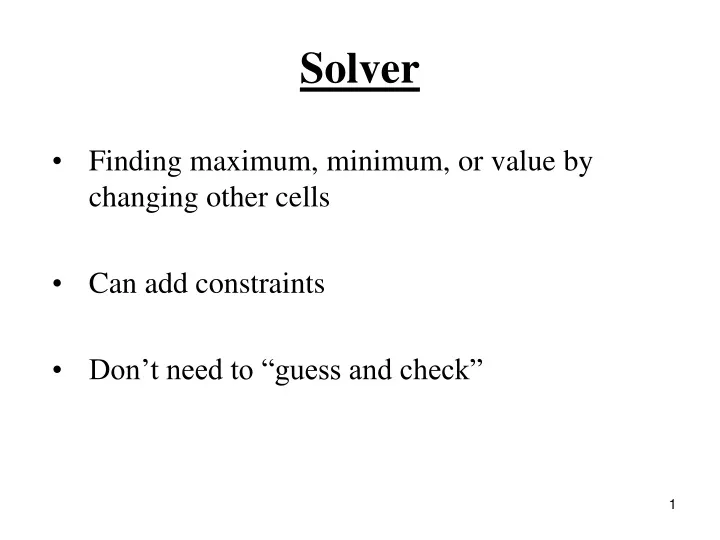
Solver. Finding maximum, minimum, or value by changing other cells Can add constraints Don’t need to “guess and check”. Solver. Using Solver, Excel’s Solver. Using Solver. Excel’s Solver. 1 . EXCEL’S SOLVER

E N D
Solver • Finding maximum, minimum, or value by changing other cells • Can add constraints • Don’t need to “guess and check”
Using Solver, Excel’s Solver Using Solver. Excel’s Solver 1. EXCEL’SSOLVER The utility Solver is one of Excel’s most useful tools for business analysis. This allows us to maximize, minimize, or find a predetermined value for the contents of a given cell by changing the values in other cells. Moreover, this can be done in such a way that it satisfies extra constraints that we might wish to impose. Example1. The size limitations on boxes shipped by your plant are as follows. (i) Their circumference is at most 100 inches. (ii) The sum of their dimensions is at most 120 inches. You would like to know the dimensions of such a box that has the largest possible volume. Let H, W, and L be the height, width, and length of a box; respectively; measured in inches. We wish to maximize the volume of the box, V = HWL, subject to the limitations that the circumference C = 2H + 2W 100 and the sum S = H + W + L 120. This problem is set up in the Excel file Shipping.xls. We will outline its solution with screen captures and directions. First, enter any reasonable values for the dimensions of the box in Cells B7:D7. Shipping.xls T C I (material continues)
Using Solver, Solver FRAGILE Crush slowly Enter cell that computes volume. Select Max. Enter cells that contain dimensions H W Click on Add. L Using Solver. Excel’s Solver: page 2 To use Solver, click on Data, then Solver in the Analysis box. In older versions of Excel select Tools in the main Excel menu, then click on Solver. To use Solver, click on Data, then Solver in the Analysis box. In older versions of Excel select Tools in the main Excel menu, then click on Solver. Computer Problem? (material continues) Shipping.xls T C I
Using Solver, Solver Using Solver. Excel’s Solver: page 3 The requirement that the circumference be at most 100 inches is called a constraint. We want to have the contents of Cell E7 be at most 100. Enter cell that computes circumference. Select <=. Click on OK. Enter the limiting number. Repeat the above process to add the constraint F7 <= 120, then click on Solve. Shipping.xls T C I (material continues)
Using Solver, Solver Using Solver. Excel’s Solver: page 4 Click on Solve. Click on Keep Solver Solution. Click on OK. Shipping.xls T C I (material continues)
Using Solver, Solver Using Solver. Excel’s Solver: page 5 The dimensions that maximize volume are now shown in Cells B8:D8. The maximum volume, the value of the circumference and the sum of the dimensions are now displayed. For a maximum volume of 43,750 cubic inches, the box should be 25 inches high, 25 inches wide, and 70 inches long. In rare cases; such as very large or small initial values of H, W, or L; you may need to add the constraints B7 >= 0, C7 >= 0 and D7 >= 0. Shipping.xls T C I (material continues)
Using Solver, Solver Using Solver. Excel’s Solver: page 6 Show ex3-sep14-shipping.xls Rush! shipping company limits the size of the boxes that it accepts by limiting their volume to at most 16 cubic feet (27,648 cubic inches). For it to ship a box, each dimension must be between 3 and 54 inches. (i) Modify Shipping.xls and use Solver to find the dimensions of a Rush! box which will accept the longest possible item. Hint: Use different initial values for each dimension. (ii) What is the maximum length of such an item? Note that the longest item which can be shipped in a box has a length of Exercise 3 Shipping.xls T C I (material continues)
Solver • Sensitive to initial value • Use graphical approximation to help solve project • Use to verify/solve Questions 1 - 3 • Use to solve Questions 6 - 8
Demand Function D(q) Revenue D(q) q q Integration • Revenue as an area under Demand function
Demand Function Total Possible Revenue Integration • Total possible revenue-The total possible revenue is the money that the producer would receive if everyone who wanted the good, bought it at the maximum price that he or she was willing to pay. This is the greatest possible revenue that a seller or producer could obtain when operating with a given demand function
Demand Function Consumer Surplus D(q) Revenue Not Sold q Integration • Consumer surplus – revenue lost by charging less/ Some buyers would have been willing pay a higher price for the good than we charged. The total extra amount of money that people who bought the good would have paid is called the consumer surplus • Producer surplus – revenue lost by charging more/ some potential customers do not buy the good, because they feel that the price is too high. The total amount of this lost income, which we will call not sold, is represented by the area of the region under the graph of the demand function to the right of the revenue rectangle.
Integration • Approximating area under graph - Counting rectangles (by hand) - Using Midpoint Sum (by hand) - Using Midpoint Sums.xls (using Excel) - Using Integrating.xls (using Excel)
Integration • Approximating area (Counting Rectangles) Ex. Approx. 9 rectangles Each rectangle is 0.25 square units Total area is approx. 2.25 square units
Integration • Approximating area (Midpoint Sums) - Notation - Meaning
Integration • Approximating area (Midpoint Sums) - Process Find endpoints of each subinterval Find midpoint of each subinterval
Integration • Approximating area (Midpoint Sums) - Process (continued) Find function value at each midpoint Multiply each by and add them all This sum is equal to
Integration • Approximating area (Midpoint Sums) Ex1. Determine where .
Integration • Approximating area (Midpoint Sums) Ex1. (Continued)
IntegrationApproximating area (Midpoint Sums.xls) =6*x-4*x^2 Ex1. (Continued)
EXAMPLE 2 - Modify sheet n = 20 in Area Example.xls, so that it computes the sum S100(f, [0, 4]), with 100 subintervals, for f(x) = 2x x2/2. • Show • ex2-n-100Area Example.xlsm
Integration-9/28 • Approximating area (Integrating.xls) - File is similar to Midpoint Sums.xls - Notation: or or …
Integrationshow ex3-Integrating.xlsm • Approximating area (Integrating.xls) Ex3. Use Integrating.xls to compute
Integration • Approximating area (Integrating.xls) Ex3. (Continued) So . Note that is the p.d.f. of an exponential random variable with parameter . This area could be calculate using the c.d.f. function .
Integration • Approximating area (Integrating.xls) Ex3. (Continued)
Integration, Integrals Where f(mi) < 0, the product f(mi)Dx is also negative. Thus, the midpoint sums will approximate the “signed area” of the region between the x-axis and the graph of f, over [a, b]. This is the algebraic sum of the area above the axis, minus the area below the axis. + b a Integration. Integrals 2. INTEGRALS What would happen if we computed midpoint sums for a function which might assume negative values in the interval [a, b]? T C I (material continues)
Integration, Integrals the integral of f over [a, b] is and it represents the algebraic sum of the signed areas of the regions between the horizontal axis and the graph of f, over [a, b].
Integration • Approximating area - Values from Midpoint Sums.xls can be positive, negative, or zero - Values from Integrating.xls can be positive, negative, or zero
Integration, Applications Integration. Applications: page 6 Revenue computations for an arbitrary demand function work in the same way as those for the buffalo steak dinners. Let D(q) give the price per unit for a good,that would result in the sale of q units, and let qmax be the maximum number of units that could be sold at any price. That is, D(qmax) = 0. The total possible revenue is given by If qsold units are sold, then the revenue will be qsoldD(qsold). The following formulas give consumer surplus and lost revenue from units not sold. It is clear that revenue + consumer surplus + not sold = total possible revenue. T C I (material continues)
Integration • Ex4. Suppose a demand function was found to be . Determine the consumer surplus at a quantity of 400 units produced and sold.
Integration • Ex. (Continued) Calculate Revenue at 400 units
Integration • Ex. (Continued) $107,508.80 – $83,569.60 = $23,939.20 So, the consumer surplus is $23,939.20
Integration • Formula for consumer surplus • Income stream - revenue enters as a stream - take integral of income stream to get total revenue
Fundamental Theorem of Calculus. For many of the functions, f, which occur in business applications, the derivative of with respect to x, is f(x). This holds for any number a and any x, such that the closed interval between a and x is in the domain of f. Integration Applications-oct1st • Fundamental Theorem of Calculus - Example : applies to p.d.f.’s and c.d.f.’s Recall from Math 115a
Integration, Applications Example4. The Plastic-Is-Us Toy Company incoming revenue -as an income stream(rather than a collection of discrete payments) At a time t years from the start of its fiscal year on July 1 the company expects to receive revenue at the rate of A(t) million dollars per year Records from past years indicate that Plastic-Is-Us can model its revenue rate A(t) = 110t5 + 330t4 330t3 + 110t2 +3.174 million dollars per year.
Integration, Applications Oct. 1 Jan. 1 April 1 July 1 July 1 8 6 A(t) 4 2 0 0 0.25 0.5 0.75 1 t The chief financial officer wants to compute the total amount of revenue that Plastic-Is-Us will receive in one year. The income stream, A(t), is a rate of change in money, given in million dollars per year. the units along the t-axis are years the area of a region under the graph of A(t) is given in (millions of dollars/year)(years) = millions of dollars.
Since gives the area between the t-axis and the graph of • A(t), over the interval [0, T], it can be shown that the integral gives the total amount of money, in millions of dollars, that will be received from the income stream in the first T years.
Integration, Applications Use Integrating.xls to compute the total income received by Plastic-Is-Us during the period from 0 to 1 year. (Remember that we must use x, not t, as the variable of integration in Integrating.xls.)
Integration, Applications The total revenue, in dollars, received from an income stream of A(t) dollars per year, starting now and continuing for the next T years is given by Suppose that money earns at an annual rate, r, compounded continuously. The present dollar value of an income stream of A(t) dollars per year, starting now and continuing for the next T years is given by Integration. Applications: page 12 In addition to the total revenue, a company would often like to know the present value of its income stream during the next T years (0 t T), assuming that money earns interest at some annual rate r, compounded continuously.
Integration, Applications Example5. We return to the Plastic-Is-Us Toy Company that we considered in Example 4. Recall that they have an income stream of A(t) = 110t5 + 330t4 330t3 + 110t2 +3.174 million dollars per year. The management of Plastic-Is-Us would like to know the present value of its income stream during the next year (0 t 1), assuming that money earns interest at an annual rate of 5.5%, compounded continuously. Applying the integral formula for present value to Plastic-Is-Us, we use Integrating.xls to find that the present value of their income stream for one year, starting on July 1, is million dollars.
Integration, Calculus Fundamental Theorem of Calculus. For many of the functions, f, which occur in business applications, the derivative of with respect to x, is f(x). This holds for any number a and any x, such that the closed interval between a and x is in the domain of f. the inverse connection between integration and differentiation is called the Fundamental Theorem of Calculus. Example 7. Let f(u) = 2 for all values of u. If x 1, then integral of f from 1 to x is the area of the region over the interval [1, x], between the u-axis and the graph of f.
Integration, Calculus (1, 2) (x, 2) 2 x 1 x In the section Properties and Applications of Differentiation, we saw that the derivative of f(x) = mx + b is equal to m, for all values of x. Thus, the derivative of with respect to x, is equal to 2. As predicted by the Fundamental Theorem of Calculus, this is also the value of f(x). The next example uses the definition of a derivative as the limit of difference quotients. The region whose area is represented by the integral is rectangular, with height 2 and width x 1. Hence, its area is 2(x 1) = 2x 2, and
Integration, Calculus Example 8. Recall the income stream of A(t) = 110t5 + 330t4 330t3 + 110t2 +3.174 million dollars per year that was expected by the Plastic-Is-Us toy company in Example 4 of Applications. Let G(T) be the total income that is expected during the first T years, for 0 T 1. Picking a time T = 0.5 years, we will check that the instantaneous rate of change of G(T), with respect to T, is the same as A(T). Note that We now wish to compute G(0.5). Recall that G(T) is approximated by the difference quotient for small values of h. We will let h = 0.0001, and use Integrating.xls to evaluate G(0.5 + 0.0001) and G(0.5 0.0001). Integrating.xls rounds the numerical values of integrals to four decimal places. For the present calculation, we gain extra precision by copying the values from Cell N20 and keeping all of their decimal places. G(0.5 + 0.0001) = G(0.5001) = 2.79078611562868 G(0.5 0.0001) = G(0.4999) = 2.78946381564699
Integration, Calculus These give a value of 6.6115 for the difference quotient rounded to four decimal places. This is the instantaneous rate of change in total income after 0.5 years. Integrating.xls shows the same value for A(0.5). Noting that we have verified the Fundamental Theorem of Calculus. At T = 0.5, the derivative of with respect to T, is equal to A(T).