Download
1 / 34
340 likes | 345 Vues
A Model of the Chromosphere: Heating, Structures, and Circulation. Paul Song Space Science Laboratory and Department of Physics, University of Massachusetts Lowell Acknolwledgments: V. M. Vasyliūnas and Jiannan Tu. The Solar Photosphere.

E N D
A Model of the Chromosphere: Heating, Structures, and Circulation Paul Song Space Science Laboratory and Department of Physics, University of Massachusetts Lowell Acknolwledgments: V. M. Vasyliūnas and Jiannan Tu
The Solar Photosphere • White light images of the Sun: granules, networks, sunspots, • The photosphere reveals interior convective motions & complex magnetic fields: β << 1 β ~ 1 β > 1
The Solar Chromosphere Images through H-alpha filter: red light (lower frequency than peak visible band) Filaments, active regions, prominences, supergranules, lanes (strong B), spicules
Type II Spicules • Thin straw-like structures, • lifetime ~ 10-300 sec. • 150-200 km in diameter • 20-150 km/s upward speed, • shoot up to 3-10 Mm • Fresh denser gas flowing from chromosphere into corona • Rooted in strong field ~ 1kG • 6000-7000 of them at a give time on the sun
1-D Empirical Chromospheric Models Vernazza, Avrett, & Loeser, 1981
The Solar Atmospheric Heating Problem(since Edlen 1943) • Explain how the temperature of the corona can reach 2~3 MK from 6000K on the surface • Explain the energy for radiation from regions above the photosphere Solar surface temperature
The Atmospheric Heating Problem, cont.(Radiative Losses) • Due to emissions radiated from regions above the photosphere • Photosphere: optical depth=1: radiation mostly absorbed and reemitted => No energy loss below the photosphere • Chromosphere: optical depth<1: radiation can go to infinity => energy radiated from the chromosphere is lost • Corona: nearly fully ionized: Little radiation is emitted and little energy is lost via radiation • Total radiative loss is R ~ N2*Tn • The temperature profile is maintained by the balance between heating and radiative loss: R=Q • Temperature increases where heating rate Q/N2 increases Corona Chromosphere Photosphere
Lower quiet Sun atmosphere (dimensions not to scale): Wine-glass or canopy-funnel shaped B field geometry: “network” and “internetwork”; “canopy” and “sub-canopy”. Network: lanes of the supergranulation, large-scale convective flows Smaller spatial scales convection: the granulation, weak-field Upward propagating and interacting shock waves, from the layers below the classical temperature minimum, Type-II spicules: above strong B regions.
Chromospheric Heating by Vertical Perturbations • Vertically propagating acoustic waves conserve flux (in a static atmosphere) • Amplitude eventually reaches Vphand wave-train steepens into a shock-train. • Shock entropy losses go into heat; only works for periods < 1–2 minutes… Bird (1964) ~ • Carlsson & Stein (1992, 1994, 1997, 2002, etc.) produced 1D time-dependent radiation-hydrodynamics simulations of vertical shock propagation and transient chromospheric heating. Wedemeyer et al. (2004) continued to 3D... (Steven Cranmer, 2009)
Something is Wrong: • With increased complexity, the fundamental problems are not resolved (not even addressed)! • Mutual assurance between simulations (with parameters that are 1000 times different from observations) and interpretations • Heating rate is 100 times too small (or waves need 100 times stronger • What forms field geometry? • What forms the temperature profile? • What forms the transition region? • What produces spicules? • Not self-consistent physical processes
Heating by Horizontal Perturbations(previous theories) Single fluid MHD: heating is due to internal “Joule” heating (evaluated correctly?) Single wave: at the frequencies of peak power, not a spectrum Weak damping: “Born approximation”, the energy flux of the perturbation is constant with height Insufficient heating (a factor of 50 too small): a result of weak damping approximation Less heating at lower altitudes Stronger heating for stronger magnetic field (?)
Required Heating (for Quiet Sun): Radiative Losses & Temperature Rise • Total radiation loss in chromosphere: 106~7 erg cm-2 s-1 . • Radiation rate: • Lower chromosphere: 10-1 erg cm-3 s-1 • Upper chromosphere: 10-2 erg cm-3 s-1 • Power to launch solar wind or to heat the corona to 2~3 MK: 3x10⁵ erg cm-2 s-1 • focus of most coronal heating models • Power to ionize: small compared to radiation • The bulk of atmospheric heating occurs in the chromosphere (not in the corona where the temperature rises) • Upper limit of available wave power ~ 108~9 erg cm-2 s-1 • Observed wave power: ~ 107 erg cm-2 s-1 • Efficiency of the energy conversion mechanisms • More heating at lower altitudes
Conditions in the Chromosphere General Comments: • Partially ionized • Neutrals produce emission • Similar to thermosphere -ionosphere • Motion is driven from below • Heating can be via collisions between plasma and neutrals Objectives: to explain • Temperature profile, especially a minimum at 600 km • Sharp changes in density and temperature at the Transition Region (TR) • Spicules: rooted from strong field regions • Wine-glass shaped magnetic field geometry • Physically self-consistent Avrett and Loeser, 2008
Plasma-neutral Interaction • Plasma (red dots) is driven with the magnetic field (solid line) perturbation from below • Neutrals do not directly feel the perturbation while plasma moves • Plasma-neutral collisions accelerate neutrals (open circles) • Longer than the neutral-ion collision time, the plasma and neutrals move nearly together with a small slippage. Weak friction/heating • On very long time scales, the plasma and neutrals move together: no collision/no heating • Similar interaction/coupling occurs between ions and electrons in frequencies below the ion collision frequency, resulting in Ohmic heating
Simplified Equations for Chromosphere(Leading terms) Faraday’s law Ampere’s law Generalized Ohm’s law Plasma momentum equation Neutral momentum equation Heating rate [Vasyliūnas and Song, JGR, 110, A02301, 2005] Ohmic/Joule Frictional
Total Heating Rate from a Power-Law Source1-D Stratified Without Vertical Flow or Current strong background field: B << B, low frequency: << ni [Song and Vasyliunas, 2011]
Tu and Song, [2013] Collisional MHD Simulation Song and Vasyliunas, [2011] Analytical • Stronger heating: • weaker B in lower region • stronger B in upper region
Perturbation in the Photosphere [Tu and Song, 2013]
[Tu and Song, 2013] Figure 7. Variation of heating rate as a function of time and altitude for B0 = 50 G. Heating rate includes both frictional and true Joule heating rates.
Figure 10. Energy flux spectra of transmitted waves calculated at z=3100 km for the ambient magnetic field B0 =10, 50, 100, 500 G. High frequency waves strongly damped and completely damped above a cutoff frequency which depends on the magnetic field (~0.014 Hz, 0.1 Hz, 0.4 Hz, and 0.7 Hz for B0 =10, 50, 100, 500 G). [Tu and Song, 2013]
Total Heating Rate Dependence on Bat the photosphere [Song and Vasyliunas, 2014] Logarithm of heating per cm, Q, as function of field strength over all frequencies in erg cm-3 s-1 assuming n=5/3, ω0/2π=1/300 sec and F0 = 107 erg cm-2 s-1.
Energy Transfer and Balance • Heating: Ohmic+frictional • Radiative loss: electromagnetic • Thermal conduction: collisional without flow • Convection/circulation: gravity/buoyancy
Importance of Thermal Conduction Energy Equation Time scale:~ lifetime of a supergranule:> ~ 1 day~105 sec Heat Conduction in Chromosphere • Perpendicular to B: very small • Parallel to B: Thermal conductivity: • Conductive heat transfer: (L~1000 km, T~ 104 K) Thermal conduction is negligible within the chromosphere: the smallness of the temperature gradient within the chromosphere and sharp change at the TR basically rule out the significance of heat conduction in maintaining the temperature profile within the chromosphere. Heat Conduction at the Transition Region (T~106 K, L~100 km): Qconduct ~ 10-6 erg cm-3 s-1: (comparable to or greater than the heating rate) important to provide for high rate of radiation
Importance of Convection Energy Equation Lower chromosphere: density is high, optical depth is significant ~ black-body radiation R~ 100 erg cm-3 s-1 (Rosseland approximation) Q~ 100 erg cm-3 s-1 (Song and Vasyliunas, 2011) Convective heat transfer: maybe significant in small scales Upper chromosphere: density is low, optical depth very small: not black-body radiation Q/Nn~~ 10-16 erg s-1 Convection, r.h.s./Nn, ~ 10-17 erg s-1 (for N~Ni~1011 cm-3, p~10-1 dyn/cm2) Convection is negligible in the chromosphere to the 0th order: Q/Nn = Temperature, T, increases with increasing Q/Nn
Heating Rate Per Particle • Heating and radiative loss balance R≈Q • Radiative loss is R ~ N(T) • Temperature is T ~(Q/N) Expected T profile • Tmin near 600 km • T is higher in upper region with strong B • T is higher in lower altitudes with weaker B B (Gauss) Logarithm of heating rate per particle Q/Ntot in erg s-1, solid lines are for unity of in/i (upper) and e/e (lower) [Song and Vasyliunas, 2014]
Chromospheric Circulation [Song and Vasyliunas, 2014] • Two (neutral) convection cells • Upper cell: driven by expansion of hotter region in strong field (networks), sunk in weaker field (internetworks) region of colder gas, and completed by continuity requirement • Lower cell: downdraft in strong field regions (consistent with Parker [1970] • B-field: wine-glass shaped • expanding in the upper region to become more uniform by convection in addition to total pressure balance • B-field: more concentrated in the lower cell as pushed by the flow
Conclusions • Based (semi-quantitatively to order of magnitude) on the 1-D analytical model that can explain the chromospheric heating • The model invokes heavily damped Alfvén waves via frictional and Ohmic heating • The damping of higher frequency waves is heavy at lower altitudes for weaker field • Only the undamped low-frequency waves can be observed above the corona (the chromosphere behaves as a low-pass filter) • More heating (per particle) occurs at lower altitudes if the field is weak and at higher altitudes if the field is strong • Extend to horizontally nonuniform magnetic field strength • Temperature is determined by the balance between heating and radiation in most regions • Temperature is higher in higher heating rate regions • Heat conduction from the coronal heating determines the temperature profile near and above transition region • The nonuniform heating drives chromospheric convection/circulation • Consistent with observed features • Circulation of Super granule size • Temperature minimum occurs in the place where there is a change in heating mechanism: electron Ohmic heating below and ion frictional heating above. • Transition region is formed when heating rate is not large enough to support radiation • Spicules are formed in regions of strong B where heating is strong in the upper region • The circulation distorts the field lines into a wine-glass shaped geometry
How to observethe chromosphere? Hβ Hα He D3 Fe XIV 5303 Ca II H & K Hγ Hα He D3 Fe XIV 5303 Hβ Hγ Ca II H & K
SDO/AIA 1600 Å IBIS Mosaic – 03 August, 2010 Ca II 8542 Å