Download
1 / 21
210 likes | 212 Vues
Explore correlations between variables and crime rates in the US, examining positive and negative associations. Discuss the limitations of simple linear regression in establishing causation.

E N D
Quantitative Methods – Week 5: Linear Regression Analysis Roman Studer Nuffield College roman.studer@nuffield.ox.ac.uk
Homework (II) • Many factors (variables) are potentially associated with the drop in crime rates in the US. Where do you find correlations between a variable and the falling crime rate? Which variables are positively, which ones negatively correlated with the crime rate variable? Where do you not find any correlation? Explanations? Concept/Variable Correlation Measured Variable Strong economy Unemployment rate, poverty level Reliance on prisons Number of prisoners Education Educational Attainment Legalizing abortion Number of abortions How did you solve the lag problem with the abortion variable?
Simple Linear Regression: Introduction • As with correlation, we are still looking at the relationship between two (ratio level) variables, but now we do not treat them symmetrically anymore, but make a distinction between the two: influences • As a consequence, the question that can be anwered with correlation analysis and regression analysis are different:
Simple Linear Regression: Introduction (II) • Therefore, we move from issues of mere association to issues of causality… • HOWEVER: A simple linear regression cannot establish causation! • We assume that causality runs from x to y • Sometimes this assumption is questionable, then more sophisticated models and tests are needed • Simultaneous equation models • Two-stage least square regressions • Causality tests • So we have to be careful when making such assumptions. Let’s look at some pairs of variables. • Which is the explanatory variable and which the dependent variable? • In which cases might you expect a mutual interaction between the two variables? • Height and weight • Birth rate and marriage rate • Rainfall and crop yield • Rate of unemployment and level of relief expenditure in British parishes • Government spending on welfare programmes and the voting share of left-liberal parties • CO2 emissions and global warming
Simple Linear Regression: Introduction (III) • Straight line (“linear”) relationship between two variables • The relationship between two variables can take a nonlinear form • Kuznets (1955) hypothesised that the relationship between the level of economic development (x) and income inequality (y) takes the form of a nonlinear (inverted-U shaped) form: Income Inequality Economic Development Multiple or multivariate regression includes two or more explanatory variables
The Equation of a Straight Line • The equation of a straight line: Y = a + bX Example: y=2+3x
The Equation of a Straight Line (II) • Equation of a straight line: Y=a+bX • Y and X are the dependent and the independent variable respectively and y1, y2, …, yn and x1, x2, …, xn their values • a is the intercept. It determines the level at which the straight line crosses the vertical axis, i.e. it gives the value of y when x=0 • b measures the slope of the line • Positive relationship: b>0 • No relationship: b=0 • Negative Relationship b<0 • If x increases by one unit, y will increase by b units
Fitting the Regression Line How do we find the line, which is the “best fit”, i.e. the line that describes the linear relationship between X and Y the best This is an issue as in the real world, relationships between two variables never follow a completely linear pattern…
Regression line IP=a+bWage =YUK- ŶUK Fitting the Regression Line (II) The regression line predicts the values of Y based on the values of X. Thus, the best line will minimise the deviation between the predicted and the actual values (the error, e)
Fitting the Regression Line (III) However, to avoid the problem that positive and negative deviations cancel out, we look at squared deviations (Yi– Ŷi)2 Also, as we want to minimise the total errors, we are interested in minimising the sum of all squared errors Therefore, the regression line it the line that…. “minimizes the sum of the squares of the vertical deviation of all pairs of the values of X and Y from the regression line” This estimation procedure is known as ordinary least squares regression (OLS). Its formal derivation yields the two formulae needed to calculate the regression line, i.e. a formula for the intercept (a) and a formula for the slope (b):
Fitting the Regression Line (IV) With these two formulae, we can actually easily calculate the regression line for small datasets by hand. However, for large datasets and when we have more than one explanatory variable, we use the Stata to do it for us
The Goodness of Fit • Once we get the “best fit” regression line, we still want to know “how good a fit” this line really is: • How much of the variation in Y is explained by this regression line? • The measure to describe the explanatory power of a regression is the coefficient of determination r2, which is equal to the square of the correlation coefficient • It is a measure of the success with which the movements in Y are explained by the movements in X • In particular it measures how much of the derivation of Y from the mean of Y is explained by the regression
The Goodness of Fit (II) • This is the interactive part of the class…. • Please explain the concept depicted in the following graph in your own words… Regression line x
The Goodness of Fit (III) Total variation = explained variation + unexplained variation TSS ESS USS R²=ESS/TSS Explained Sum of Squares/Total Sum of Squares
The Goodness of Fit (IV) • R2 gives the proportion of the sample variation in y that is explained by x • R2 =0.35 means that the explanatory variable explains 35% of the variation in the dependent variable • R2 ranges between 0 and 1 • The higher R2 the better the fit of the regression line to the data • R2 can be used to compare the explanatory power of different regression models (with the same dependent variable) • R2 has to be interpreted in the light of what we would expect • A low R2 does not necessarily mean that an OLS regression equation is useless
Computer Class: • Regression Analysis
Exercises • Weimar elections: Unemployment and votes for the Nazi A) Descriptive Statistics Get the dataset about the Weimar election of 1932 at http://www.nuff.ox.ac.uk/users/studer/teaching.htm • Look at the variables (votes for the Nazi party, level of unemployment) in turn • Get a first visualisation of the data; does it look normally distributed? • Compute the mean, median, standard deviation, coefficient of variation, kurtosis and skewness for the variable • Make a scatter plot; Do you think the two variables are associated? How and how strongly? B) Regression Analysis • Which one is the dependent variable? • Estimate the regression line • What is the interpretation? • What is the explanatory power of the regression? • Draw a scatter plot and add the regression line
Exercises (II) 2. Weimar elections: Nazi votes and the share of Catholics Do the same exercises as with the unemployment rate A) Descriptive Statistics B) Regression Analysis
Appendix: STATA Commands • regress depvar indepvars Linear regression; the dependent and independent variables are indicated by the order. The dependent variable depvar comes first, then the independent variable(s) indepvar follow • predict yhat, xb Calculates the linear prediction for each observation, i.e. yhati= a+b*indepvari • predict res, resid The option “resid” behind the comma let STATA calculate and save the residuals, i.e. resi=yi- yhati • generate newvar=exp Creates a new variable. STATA provides numerous functions, see STATA’s Help on “Functions and expressions”/“math functions
Homework • Readings: • Feinstein & Thomas, Ch. 5 • Problem Set 4: • Finish the exercises from today’s computer class if you haven’t done so already. Include all the results and answers in the file you send me • On the next slide you see part of the macroeconomic dataset we used in week 3. Look at the variables “GDP per head” and “education”, assuming that GDP per head is the dependent variable and education the explanatory variable. Calculate by hand: • The regression coefficient, b • The intercept, a • The total sum of squares • The explained sum of squares • The residual sum of squares • The coefficient of determination (hint: graph the values first by hand and then look at tables 4.1 and 4.2) • Download the complete data set at http://www.nuff.ox.ac.uk/users/studer/teaching.htm(“macro data”) and calculate the regression line and the coefficient of determination • Interpret the results • Do the results differ from the correlation results?