Download
1 / 1
10 likes | 73 Vues
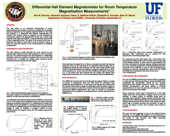
Centimeter interval notches. Four rods fixed into the sample mount secure to the Hall elements’ board, which in turn fasten into the PVC probe. Three sets of twisted pairs connect to electronics on workbench. Hall elements. z- axis. Sample.

E N D
Centimeter interval notches Four rods fixed into the sample mount secure to the Hall elements’ board, which in turn fasten into the PVC probe Three sets of twisted pairs connect to electronics on workbench Hall elements z-axis Sample Differential Hall Element Magnetometer for Room Temperature Magnetization Measurements* Alex M. Sincore, Alejandro Quintero Cabra, S. Matthew Gilbert, Elisabeth S. Knowles, Mark W. Meisel Department of Physics and NHMFL, University of Florida, Gainesville, FL Probe mount painted Gator for pride OVERVIEW: The Hall effect is an important characteristic of some semiconductors that develop a transverse voltage that is typically linearly proportional to the applied magnetic fields [1]. By using this property in a differential Hall element magnetometer, the coercive and remnant fields of materials can be measured by inserting the sample and magnetometer device into a static, high magnetic field region provided by a superconducting solenoid with a room temperature bore. The goal of the present work was to determine the signal to noise ratio in order to provide a figure of merit for using this system for the characterization of magnetic nanoparticles. EXPERIMENTAL SETUP AND METHOD: The Hall elements, model HG-166A [2], were chosen for the magnetometer because of their high sensitivity (2 V per T) and their low cost. The method employs two Hall elements in a differential schematic, where the sample is localized next to one of the Hall elements [Fig. 1]. Ideally, the voltage being measured arises exclusively from the presence of the sample. Fig. 1: Differential Hall Element Magnetometer Circuit Diagram. The power supply and multimeters connect to LabVIEW via GPIB-USB-HS. The dual op-amp model is LM-358AN [3]. The Differential Hall Element Magnetometer (DHEM) is fixed at the end of a PVC probe that is designed to enter the superconducting magnet at centimeter intervals [Fig. 2]. Twisted pairs of copper wire (40 AWG) connect the DHEM to a workbench where the electronics are located. A LabVIEW program was written that regulates the DC voltage in order to maintain a constant current of 5mA. Simultaneously, the program stores the Hall voltage measured at each interval. Fig. 2: Left: Schematic diagram of probe. Right: Picture of workstation with probe inserted into the superconducting magnet. Characterizing the magnet [Fig. 3] allows a standard by which the distance along the z-axis can be converted to an appropriate field strength. Due to irregularities among the Hall elements, the two most similar profiles were chosen to minimize background readings. A chunk of magnet (from a 1970’s stereo speaker) [Fig. 4]was mounted to the DHEM and brought to saturation at 2 T. The probe was then removed and the sample was flipped, thus beginning the hysteresis curve at the corresponding remnant magnetization. DATA AND RESULTS: The DHEM was inserted and removed through the magnet without a sample to provide a background noise plot that would be subtracted from subsequent data analysis [Fig. 5]. The mass of the sample was reduced until the coercive field would no longer be detectable, which provides a figure of merit for how much of a material is needed to effectively employ the DHEM. A commercial SQUID magnetometer was used to provide an alternative measurement for the purpose of comparing them to those obtained by the DHEM [Fig. 6]. Fig. 7: Hysteresis plots (from remnant magnetization to saturation, then immediately back to remnant for time purposes) for descending sample mass. The measured coercive field values [Fig. 7] fall within 10%, except for the 240mg sample which is within 18% (not pictured) of the SQUID’s analysis. A slope arises at approximately 750 mT that is attributed to unknown reasons, though presumably due to the non-linear growth seen in the background noise plot. Conversion from millivolts to emu G was accomplished by matching the remnant magnetization values from the DHEM and SQUID and calculating a ratio, which in turn was 1 mV ≈ 0.256 emu G. CONCLUSIONS AND FUTURE WORK: The use of a DHEM to measure the coercive fields of materials is a time and cost efficient substitute to using the SQUID. After considering the uncertainties created by the: irregular background noise (ideally should be linear), error between identical measurements, and offset voltage; a minimum magnetization of ≈2 emu G is necessary for precision results due to the sensitivity of the DHEM. Future endeavors would entail construction of a new light weight probe and incorporating a stepper motor for interval readings. A simple change to LabVIEW would allow an automatic data acquisition without manual interference. Also, exploration into minimizing background noise (experiment with different Hall elements) and the cause of the extraneous slope would help to increase accuracy and precision. In order to increase the figure of merit, more sensitive units would be required. *ACKNOWLDGEMENTS: This work has been supported, in part, by the National Science Foundation via the NHMFL REU Program, the UF Department of Physics REU, and DMR-0701400 (MWM). We gratefully acknowledge the receipt of Hall elements from GMW Associates <http://www.gmw.com/index.html>. REFERENCES: [1] Kittel, Charles (1976). Introduction to Solid State Physics (5th ed.). John Wiley & Sons, Inc. [2] HG-166A Datasheet <http://www.asahi-kasei.co.jp/ake/en/product/hall/file/hg-166a_e.pdf> [3] LM-358AN Datasheet <http://www.national.com/ds/LM/LM158.pdf> Maximum magnetic field located at 56-58cm into bore Fig. 4: Speaker magnet chunks used. Left to right (mg): 620, 240, 130, 55, 30 (in a gel capsule), 10. 1.1 cm 0.3 cm Fig. 5: Magnet characterized by the DHEM without a sample. Subtracted from measurements as background noise. Fig. 3: Magnetic Field vs. Distance of the super-conducting magnet (set at 2 T), determined by averaging 10 HG-166A single Hall elements’ results. Fig. 6: SQUID analysis of a chunk of speaker magnet.