Download
1 / 41
410 likes | 418 Vues
This talk explores the marriage of high-dimensional machine learning techniques with modern linguistic representations for landmark-based speech recognition. The goal is to test globally optimized computational models of speech psychology as automatic speech recognizers.

E N D
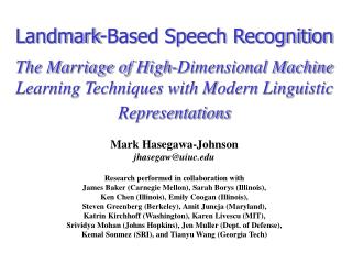
Landmark-Based Speech RecognitionThe Marriage of High-Dimensional Machine Learning Techniques with Modern Linguistic Representations Mark Hasegawa-Johnson jhasegaw@uiuc.edu Research performed in collaboration with James Baker (Carnegie Mellon), Sarah Borys (Illinois), Ken Chen (Illinois), Emily Coogan (Illinois), Steven Greenberg (Berkeley), Amit Juneja (Maryland), Katrin Kirchhoff (Washington), Karen Livescu (MIT), Srividya Mohan (Johns Hopkins), Jen Muller (Dept. of Defense), Kemal Sonmez (SRI), and Tianyu Wang (Georgia Tech)
Goal of this Talk • Experiments with human subjects (since 1910 at Bell Labs, since 1950 at Harvard) give us detailed knowledge of human speech perception. • Human speech perception is multi-resolution, like progressive JPEG: • syllables and prosody → distinctive features → words • Automatic speech recognition (ASR) works best if all parameters in the system can be simultaneously learned in order to adjust a global optimality criterion • In 1967, it became possible to globally optimize all parameters of a very simple recognition model called the hidden Markov model • Multi-resolution speech models could not be globally optimized • Therefore from 1985-1999, standard ASR ignored results from speech psychology • In the 1990s, new results in machine learning made it possible to globally optimize a multi-resolution model of speech psychology, and to use the resulting model as an automatic speech recognizer • We do not yet know how best to “marry” speech psychology with new machine learning technology • Goal of this talk: to test globally optimized computational models of speech psychology as automatic speech recognizers
What are Landmarks? • Time-frequency regions of high mutual information between phone and signal (maxima of I(phone label; acoustics(t,f)) ) • Acoustic events with similar importance in all languages, and across all speaking styles • Acoustic events that can be detected even in extremely noisy environments Where do these things happen? • Syllable Onset ≈ Consonant Release • Syllable Nucleus ≈ Vowel Center • Syllable Coda ≈ Consonant Closure I(phone;acoustics) experiment: Hasegawa-Johnson, 2000
Landmark-Based Speech Recognition Lattice hypothesis: … backed up … Words Times Scores Pronunciation Variants: … backed up … … backtup .. … back up … … backt ihp … … wackt ihp… … ONSET ONSET Syllable Structure NUCLEUS NUCLEUS CODA CODA
Talk Outline Overview • Acoustic Modeling • Speech data and acoustic features • Landmark detection • Estimation of real-valued “distinctive features” using support vector machines (SVM) • Pronunciation Modeling • A Dynamic Bayesian network (DBN) implementation of Articulatory Phonology • A Discriminative Pronunciation model implemented using Maximum Entropy (MaxEnt) • Technological Evaluation • Rescoring of word lattice output from an HMM-based recognizer • Errors that we fixed: Channel noise, Laughter, etcetera • New errors that we caused: Pronunciation models trained on 3 hours can’t compete with triphone models trained on 3000 hours. • Future Plans
Overview • History • Research described in this talk was performed between June 30 and August 17, 2004, at the Johns Hopkins summer workshop WS04 • Scientific Goal • To use high-dimensional machine learning technologies (SVM, DBN) to create representations capable of learning, from data, the types of speech knowledge that humans exhibit in psychophysical speech perception experiments • Technological Goal • Long-term: To create a better speech recognizer • Short-term: lattice rescoring, applied to word lattices produced by SRI’s NN/HMM hybrid
Overview of Systems to be Described Rescoring: Log-Linear Score Combination p(MFCC,PLP|word), p(word|words) p(SVM|word) First-Pass ASR Word Lattice word label, start & end times Pronunciation Model (DBN or MaxEnt) p(landmark|SVM) … … Acoustic Model: SVMs concatenate 4-15 frames MFCC (5ms & 1ms frame period), Formants, Phonetic & Auditory Model Parameters
I. Acoustic Modeling • Goal: Learn precise and generalizable models of the acoustic boundary associated with each distinctive feature. • Methods: • Large input vector space (many acoustic feature types) • Regularized binary classifiers (SVMs) • SVM outputs “smoothed” using dynamic programming • SVM outputs converted to posterior probability estimates once/5ms using histogram
Acoustic and Auditory Features • MFCCs, 25ms window (standard ASR features) • Spectral shape: energy, spectral tilt, and spectral compactness, once/millisecond • Noise-robust MUSIC-based formant frequencies, amplitudes, and bandwidths (Zheng & Hasegawa-Johnson, ICSLP 2004) • Acoustic-phonetic parameters (Formant-based relative spectral measures and time-domain measures; Bitar & Espy-Wilson, 1996) • Rate-place model of neural response fields in the cat auditory cortex (Carlyon & Shamma, JASA 2003)
What are Distinctive Features? What are Landmarks? • Distinctive feature = • a binary partition of the phonemes (Jakobson, 1952) • … that compactly describes pronunciation variability (Halle) • … and correlates with distinct acoustic cues (Stevens) • Landmark = Change in the value of a Manner Feature • [+sonorant] to [–sonorant], [–sonorant] to [+sonorant] • 5 manner features: [consonantal, continuant, syllabic, silence] • Place and Voicing features: SVMs are only trained at landmarks • Primary articulator: lips, tongue blade, or tongue body • Features of primary articulator: anterior, strident • Features of secondary articulator: nasal, voiced
Landmark Detection using Support Vector Machines (SVMs) False Acceptance vs. False Rejection Errors, TIMIT, per 10ms frame SVM Stop Release Detector: Half the Error of an HMM (1) Delta-Energy (“Deriv”): Equal Error Rate = 0.2% (2) HMM (*): False Rejection Error=0.3% (3) Linear SVM: EER = 0.15% (4) Radial Basis Function SVM: Equal Error Rate=0.13% Niyogi & Burges, 1999, 2002
Dynamic Programming Smooths SVMs • Maximize Pi p( features(ti) | X(ti) ) p(ti+1-ti | features(ti)) • Soft-decision “smoothing” mode: • p( acoustics | landmarks ) computed, fed to pronunciation model
Cues for Place of Articulation:MFCC+formants + ratescale, within 150ms of landmark
Soft-Decision Landmark Probabilities Kernel: Transform to Infinite- Dimensional Hilbert Space SVM Discriminant Dimension = argmin(error(margin)+1/width(margin) SVM Extracts a Discriminant Dimension Niyogi & Burges, 2002: p(class|acoustics) ≈ Sigmoid Model in Discriminant Dimension OR Juneja & Espy-Wilson, 2003: p(class|acoustics) ≈ Histogram in Discriminant Dimension
Soft Decisions once/5ms:p ( manner feature d(t) | Y(t) )p( place feature d(t) | Y(t), t is a landmark ) 2000-dimensional acoustic feature vector SVM Discriminant yi(t) Histogram Posterior probability of distinctive feature p(di(t)=1 | yi(t))
II. Pronunciation Modeling • Goal: Represent a large number of pronunciation variants, in a controlled fashion, using distinctive features. Pick out the distinctive features that are most important for each word recognition task. • Methods: • Distinctive feature based lexicon + dynamic programming alignment • Dynamic Bayesian Network model of Articulatory Phonology (articulation-based pronunciation variability model) • MaxEnt search for lexically discriminative features (perceptually based “pronunciation model”)
1. Distinctive-Feature Based Lexicon • Merger of English Switchboard and Callhome dictionaries • Converted to landmarks using Hasegawa-Johnson’s perl transcription tools Landmarks in blue, Place and voicing features in green. AGO(0.441765) +syllabic+reduced +back AX +–continuant +– sonorant+velar +voiced G closure –+continuant –+sonorant +velar +voiced G release +syllabic–low –high +back +round +tense OW AGO(0.294118) +syllabic+reduced –back IX –+continuant –+sonorant+velar +voiced G closure –+continuant –+sonorant+velar +voiced G release +syllabic–low –high +back +round +tense OW
Dynamic Programming Lexical Search • Choose the word that maximizes • Pi p( features(ti) | X(ti) ) p(ti+1-ti | features(ti)) p(features(ti)|word)
TB-LOC VELUM TT-LOC LIP-OP TB-OPEN TT-OPEN VOICING 2. Articulatory Phonology • Many pronunciation phenomena can be parsimoniously described as resulting from asynchrony and reduction of sub-phonetic features • One set of features based on articulatory phonology [Browman & Goldstein 1990]: • warmth [w ao r m p th] - Phone insertion? • I don’t know[ah dx uh_n ow_n] - Phone deletion?? • several[s eh r v ax l] - Exchange of two phones??? • instruments[ih_n s ch em ih_n n s] everybody[eh r uw ay]
. . . = = - = 1 ; 2 1 2 Pr( async a ) Pr(| ind ind | a ) given by baseform pronunciations = 1 = 1 0 1 2 3 4 … 0 .7 .2 .1 0 0 … 1 0 .7 .2 .1 0 … 2 0 0 .7 .2 .1 … … … … … … … … Dynamic Bayesian Network Model(Livescu and Glass, 2004) • The model is implemented as a dynamic Bayesian network (DBN): • A representation, via a directed graph, of a distribution over a set of variables that evolve through time • Example DBN with three features:
The DBN-SVM Hybrid Developed at WS04 Word LIKE A Canonical Form … Tongue closed Tongue Mid Tongue front Tongue open … Surface Form Tongue front Semi-closed Tongue Front Tongue open … Manner Glide Front Vowel Place Palatal … SVM Outputs p( gPGR(x) | palatal glide release) p( gGR(x) | glide release ) x: Multi-Frame Observation including Spectrum, Formants, & Auditory Model …
3. Discriminative Pronunciation Model • Rationale: baseline HMM-based system already provides high-quality hypotheses • 1-best error rate from N-best lists: 24.4% (RT-03 dev set) • oracle error rate: 16.2% • Method: Use landmark detection only where necessary, to correct errors made by baseline recognition system • Example: fsh_60386_1_0105420_0108380 Ref: that cannot be that hard to sneak onto an airplane Hyp: they can be a that hard to speak on an airplane
that can *DEL* on sneak an airplane be hard to speak onto a they can’t Identifying Confusable Hypotheses • Use existing alignment algorithms for converting lattices into confusion networks (Mangu, Brill & Stolcke 2000) • Hypotheses ranked by posterior probability • Generated from n-best lists without 4-gram or pronunciation model scores( higher WER compared to lattices) • Multi-words (“I_don’t_know”) were split prior to generating confusion networks
Identifying Confusable Hypotheses • How much can be gained from fixing confusions? • Baseline error rate: 25.8% • Oracle error rates when selecting correct word from confusion set:
Selecting Relevant Landmarks • Not all landmarks are equally relevant for distinguishing between competing word hypotheses (e.g. vowel features irrelevant for sneak vs. speak) • Using all available landmarks might deteriorate performance when irrelevant landmarks have weak scores (but: redundancy might be useful) • Automatic selection algorithm • Should optimally distinguish set of confusable words (discriminative) • Should rank landmark features according to their relevance for distinguishing words (i.e. output should be interpretable in phonetic terms) • Should be extendable to features beyond landmarks
Maximum-Entropy Landmark Selection • Convert each word in confusion set into fixed-length landmark-based representation using idea from information retrieval: • Vector space consisting of binary relations between two landmarks • Manner landmarks: precedence, e.g. V < Son. Cons. • Manner & place features: overlap, e.g. V o +high • preserves basic temporal information • Words represented as frequency entries in feature vector • Not all possible relations are used (phonotactic constraints, place features detected dependent on manner landmarks) • Dimensionality of feature space: 40 - 60 • Word entries derived from phone representation plus pronunciation rules
Maximum-Entropy Discrimination • Use maxent classifier • Here: y = words, x = acoustics, f = landmark relationships • Why maxent classifier? • Discriminative classifier • Possibly large set of confusable words • Later addition of non-binary features • Training: ideally on real landmark detection output • Here: on entries from lexicon (includes pronunciation variants)
Maximum-Entropy Discrimination • Example: sneak vs. speak • Different model is trained for each confusion set landmarks can have different weights in different contexts speak SC ○ +blade -2.47 FR < SC -2.47 FR < SIL 2.11 SIL < ST 1.75 ….. sneak SC ○ +blade 2.47 FR < SC 2.47 FR < SIL -2.11 SIL < ST -1.75 …..
Landmark Queries • Select N landmarks with highest weights • Ask landmark detection module to produce scores for selected landmarks within word boundaries given by baseline system • Example: sneak 1.70 1.99 SC ○ +blade ? Landmark detectors Confusion networks sneak 1.70 1.99 SC ○ +blade 0.75 0.56
Acoustic Feature Selection 1. Accuracy per Frame (%), Stop Releases only, NTIMIT 2. Word Error Rate: Lattice Rescoring, RT03-devel, One Talker (WARNING: this talker is atypical.)Baseline: 15.0% (113/755)Rescoring, place based on: MFCCs + Formant-based params: 14.6% (110/755) Rate-Scale + Formant-based params: 14.3% (108/755)
I don’t know DBN-SVM: Models Nonstandard Phones /d/ becomes flap /n/ becomes a creaky nasal glide
DBN-SVM Design Decisions • What kind of SVM outputs should be used in the DBN? • Method 1 (EBS/DBN): Generate landmark segmentation with EBS using manner SVMs, then apply place SVMs at appropriate points in the segmentation • Force DBN to use EBS segmentation • Allow DBN to stray from EBS segmentation, using place/voicing SVM outputs whenever available • Method 2 (SVM/DBN): Apply all SVMs in all frames, allow DBN to consider all possible segmentations • In a single pass • In two passes: (1) manner-based segmentation; (2) place+manner scoring • How should we take into account the distinctive feature hierarchy? • How do we avoid “over-counting” evidence? • How do we train the DBN (feature transcriptions vs. SVM outputs)?
DBN-SVM Rescoring Experiments • For each lattice edge: • SVM probabilities computed over edge duration and used as soft evidence in DBN • DBN computes a score S P(word | evidence) • Final edge score is a weighted interpolation of baseline scores and EBS/DBN or SVM/DBN score
Discriminative Pronunciation Model RT-03 dev set, 35497 Words, 2930 Segments, 36 Speakers (Switchboard and Fisher data) • Rescored: product combination of old and new prob. distributions, weights 0.8 (old), 0.2 (new) • Correct/incorrect decision changed in about 8% of all cases • Slightly higher number of fixed errors vs. new errors
Analysis • When does it work? • Detectors give high probability for correct distinguishing feature • When does it not work? • Problems in lexicon representation • Landmark detectors are confident but wrong mean (correct) vs. me (false) V < +nasal 0.76 once (correct) vs. what (false): Sil ○ +blade 0.87 can’t [kæ̃t] (correct) vs cat (false): SC ○ +nasal 0.26 like (correct) vs. liked (false): Sil ○ +blade 0.95
Analysis • Incorrect landmark scores often due to word boundary effects, e.g.: • Word boundaries given by baseline system may exclude relevant landmarks or include parts of neighbouring words • DBN-SVM system also failed when word boundaries grossly misaligned he much she
Conclusions • SVMs work best when: • Mixed training data, at least 3000 landmarks/class • Manner classification: Small acoustic feature vectors OK (3-20 dimensions) • Place classification: Large acoustic feature vectors best (~2000 dimensions) • DBN-SVM correctly models non-canonical pronunciations • DBN is able to match nasalized glide in place of /n/ • One talker laughed a lot while speaking; DBN-SVM reduced WER for that talker • Both DBN-SVM and MaxEnt need more training data • Our training data: 3.5 hours. Baseline HMM training data: 3000 hours. • DBN-SVM novel errors: mostly pronunciation unexpected pronunciations • MaxEnt model currently defines a “lexically discriminative” feature by comparing dictionary entries, therefore it fails most frequently when observing pronunciation variants. • MaxEnt model should instead be trained using automatic landmark transcriptions of confusable words from a large training corpus. • Both DBN-SVM and MaxEnt are sensitive to word boundary time errors. Solution: Probabilistic word boundary times?