Download
1 / 29
290 likes | 474 Vues
Chapter V: Indexing & Searching. Information Retrieval & Data Mining Universität des Saarlandes, Saarbrücken Winter Semester 2011/12. Chapter V: Indexing & Searching*. V.1 Indexing & Query processing Inverted indexes, B + -trees, merging vs. hashing,

E N D
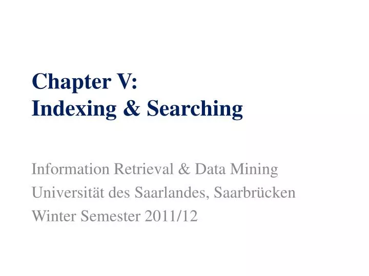
Chapter V:Indexing & Searching Information Retrieval & Data Mining Universität des Saarlandes, Saarbrücken Winter Semester 2011/12
Chapter V: Indexing & Searching* V.1 Indexing & Query processing Inverted indexes, B+-trees, merging vs. hashing, Map-Reduce & distribution, index caching V.2 Compression Dictionary-based vs. variable-length encoding, Gamma encoding, S16, P-for-Delta V.3 Top-k Query Processing Heuristic top-k approaches,Fagin’s family of threshold-algorithms, IO-Top-k, Top-k with incremental merging, and others V.4 Efficient Similarity Search High-dimensional similarity search, SpotSigs algorithm, Min-Hashing & Locality Sensitive Hashing (LSH) *mostly following Chapters 4 & 5 from Manning/Raghavan/Schütze and Chapter 9 from Baeza-Yates/Ribeiro-Netowith additions from recent research papers IR&DM, WS'11/12
...... ..... ...... ..... Server farms with 10 000‘s (2002) – 100,000’s (2010) computers, distributed/replicated data in high-performance file system (GFS,HDFS,…), massive parallelism for query processing (MapReduce, Hadoop,…) V.1 Indexing - Web, intranet, digital libraries, desktop search - Unstructured/semistructured data extract & clean index search rank present crawl handle dynamic pages, detect duplicates, detect spam fast top-k queries, query logging, auto-completion GUI, user guidance, personalization scoring function over many data and context criteria strategies for crawl schedule and priority queue for crawl frontier build and analyze Web graph, index all tokens or word stems IR&DM, WS'11/12
...... ..... ...... ..... Surfing Internet Cafes ... Surf Internet Cafe ... Surf Wave Internet WWW eService Cafe Bistro ... Extraction of relevant words Linguistic methods: stemming, lemmas Statistically weighted features (terms) Indexing Thesaurus (Ontology) Index (B+-tree) Synonyms, Sub-/Super- Concepts ... Bistro Cafe URLs Content Gathering and Indexing Bag-of-Words representations Crawling Web Surfing: In Internet cafes with or without Web Suit ... Documents IR&DM, WS'11/12
Similarity metric: (e.g., Cosine measure) Ranking by descending relevance Vector Space Model for Relevance Ranking Search engine Query (set of weighted features) Documents are feature vectors (bags of words) Using, e.g., tf*idf as weights e.g., using: IR&DM, WS'11/12
Ranking functions: • Low-dimensional queries (ad-hoc ranking, Web search): • BM25(F), authority scores, recency, document structure, etc. • High-dimensional queries (similarity search): • Cosine, Jaccard, Hamming on bitwise signatures, etc. + Dozens of more features employed by various search engines Combined Ranking with Content & Links Structure Ranking by descending relevance & authority Search engine Query (set of weighted features) IR&DM, WS'11/12
Digression: Basic Hardware Considerations 16 GB/s (64bit@2GHz) Typical Computer CPU Bus system (32–256 bits @200–800 MHz) ... ... 300 MB/s (SATA-300) M C 3,200 MB/s (DDR-SDRAM @200MHz) HD Secondary Storage 6,400 MB/s – 12,800 MB/s (DDR2, dual channel, 800MHz) Tertiary Storage HD TransferRate= width (number of bits) x clock rate x data per clock / 8 (bytes/sec) typically 1 IR&DM, WS'11/12
Moore’s Law Source: http://en.wikipedia.org/wiki/Moore%27s_law IR&DM, WS'11/12 Gordon Moore (Intel) anno 1965: “The density of integrated circuits (transistors) will double every 18 months!” → Has often been generalized to clock rates of CPUs, disk & memory sizes, etc. → Still holds today for integrated circuits!
More Modern View on Hardware Multi-core- multi-CPU Computer CPU CPU CPU CPU CPU CPU CPU CPU ... L1/L2 L1/L2 ... ... C M CPU-to-L1-Cache: 3-5 cycles initial latency, then “burst” mode HD Secondary Storage CPU-to-L2-Cache: 15-20 cycles latency HD CPU-to-Main-Memory: ~200 cycles latency IR&DM, WS'11/12 CPU-cache becomes primary storage! Main-memory becomes secondary storage!
Data Centers IR&DM, WS'11/12 Google Data Center anno 2004 Source: J. Dean: WSDM 2009 Keynote
Different Query Types Find relevant docs by list processing on inverted indexes Conjunctive queries: all words in q = q1 … qk required Disjunctive (“andish”) queries: subset of q words qualifies, more of q yields higher score • Including variant: • scan & merge • only subset of qi lists • lookup long • or negated qi lists • only for best result • candidates Mixed-mode queries and negations: q = q1 q2 q3 +q4 +q5 –q6 Phrase queries and proximity queries: q = “q1 q2 q3” q4 q5 … Vague-match(approximate)queries with tolerance to spelling variants see Chapter III.5 Structured queries and XML-IR //article[about(.//title, “Harry Potter”)]//sec IR&DM, WS'11/12
Indexing with Inverted Lists Vector space model suggests term-document matrix, but data is sparse and queries are even very sparse. Better use inverted index lists with terms as keys for B+ tree. q: {professor research xml} B+ tree on terms ... ... professor research xml 17: 0.3 17: 0.3 12: 0.5 11: 0.6 index lists with postings (docId, score) sorted by docId 44: 0.4 44: 0.4 14: 0.4 17: 0.1 17: 0.1 Google: >10 Mio. terms > 20 Bio. docs > 10 TB index 52: 0.1 28: 0.1 28: 0.7 ... 53: 0.8 44: 0.2 44: 0.2 55: 0.6 51: 0.6 ... 52: 0.3 ... terms can be full words, word stems, word pairs, substrings, N-grams, etc. (whatever “dictionary terms” we prefer for the application) • Index-list entries in docId orderfor fast Boolean operations • Many techniques for excellent compressionof index lists • Additional position index needed for phrases, proximity, etc. • (or other pre-computed data structures) IR&DM, WS'11/12
B+-Tree Index for Term Dictionary [A-I] [J-Z] m = 3 Keywords [A-Z] [J-K] [L-Q] [R-Z] [A-D] [E-F] [G-I] [A-B] [C] [D] [G] [H] [I] … … … [E] [F] IR&DM, WS'11/12 B-tree: balanced tree with internal nodes of ≤m fan-out B+-tree: leaf nodes additionally linked via pointers for efficient range scans For term dictionary: Leaf entries point to inverted list entries on local disk and/or node in compute cluster
Inverted Index for Posting Lists Documents:d1, …, dn Index-list entries usually stored in ascending order of docId (for efficient merge joins) or in descending order of per-term score (impact-ordered lists for top-kstyle pruning). Usually compressed and divided into block sizes which are convenient for disk operations. d10 s(t1,d1) = 0.9 … s(tm,d1) = 0.2 sort Index lists d10 0.9 d23 0.8 d54 0.8 d67 0.7 d88 0.2 t1 … d10 0.8 d12 0.6 d17 0.6 d23 0.2 d78 0.1 t2 … d10 0.7 d12 0.5 d23 0.4 d88 0.2 d99 0.1 t3 … IR&DM, WS'11/12
Query Processing on Inverted Lists index lists with postings (docId, score) sorted by docId q: {professor research xml} B+ tree on terms ... ... professor research xml 17: 0.3 17: 0.3 12: 0.5 11: 0.6 44: 0.4 44: 0.4 14: 0.4 17: 0.1 17: 0.1 52: 0.1 28: 0.1 28: 0.7 Given: query q = t1 t2 ... tz with z (conjunctive) keywords similarity scoring function score(q,d) for docs dD, e.g.: with precomputed scores (index weights) si(d) for which qi≠0 Find: top-k results for score(q,d) =aggr{si(d)}(e.g.: iqsi(d)) ... 53: 0.8 44: 0.2 44: 0.2 55: 0.6 51: 0.6 ... 52: 0.3 ... Join-then-sort algorithm: top-k ( [term=t1] (index) DocId [term=t2] (index) DocId ... DocId [term=tz] (index) order by s desc) IR&DM, WS'11/12
Index List Processing by Merge Join Keep L(i) in ascending order of doc ids. Delta encoding: compress Li by actually storing the gaps between successive doc ids (or using some more sophisticated prefix-free code). QP may start with those Li lists that are short and have high idf. → Candidates need to be looked up in other lists Lj. To avoid having to uncompress the entire list Lj, Lj is encoded into groups (i.e., blocks) of compressed entries with a skip pointer at the start of each block sqrt(n) evenly spaced skip pointers for list of length n. Li … 2 4 9 16 59 66 128 135 291 311 315 591 672 899 skip! Lj … 1 2 3 5 8 17 21 35 39 46 52 66 75 88 IR&DM, WS'11/12
Index List Processing by Hash Join Keep Li in ascending order of scores (e.g., TF*IDF). Delta Encoding:compress Li by storing the gaps between successive scores (often combined with variable-length encoding). QP may start with those Li lists that are short and have high scores, schedule may vary adaptively to scores. → Candidates can immediately be looked up in other lists Lj. → Can aggregate candidate scores on-the-fly. Li … 66 2 672 4 899 128 135 1591 16 315 59 291 311 Lj … 75 1 17 2 52 66 88 3 672 5 8 21 35 39 ? IR&DM, WS'11/12
Index Construction and Updates • Index construction: • extract (docId, termId, score) triples from docs • can be partitioned & parallelized • scores need idf (estimates) • sort entries termId (primary) and docId (secondary) • disk-based merge sort (build runs, write to temp, merge runs) • can be partitioned & parallelized • load index from sorted file(s), using large batches for disk I/O, • compress sorted entries (delta-encoding, etc.) • create dictionary entries for fast access during query processing • Index updating: • collect large batches of updates in separate file(s) • periodically sort these files and merge them with index lists IR&DM, WS'11/12
Map-Reduce Parallelism for Index Building a..c a..c sort merge ... ... Inverter Extractor u..z u..z sort a b … z merge a b c a d ... u f merge f a..c a..c sort z y t Inverter ... ... Extractor u..z u..z sort merge input files Map Reduce output files Intermediate files IR&DM, WS'11/12
Map-Reduce Parallelism • Programming paradigm and infrastructure • for scalable, highly parallel data analytics. • can run on 1000’s of computers • with built-in load balancing & fault-tolerance • (automatic scheduling & restart of worker processes) Easy programming with key-value pairs: Map function: KV (L W)* (k1, v1) | (l1,w1), (l2,w2), … Reduce function: L W* W* l1, (x1, x2, …) | y1, y2, … • Examples: • Index building: K=docIds, V=contents, L=termIds, W=docIds • Click log analysis: K=logs, V=clicks, L=URLs, W=counts • Web graph reversal: K=docIds, V=(s,t) outlinks, L=t, W=(t,s) inlinks IR&DM, WS'11/12
Map-Reduce Example for Inverted Index Construction class Reducer • procedure REDUCE(term t, postings [<n1,f1>, <n2,f2>, …]) • P ← new List<posting> • For posting <n, f> postings [<n1,f1>, <n2,f2>, …] do// globalidf aggregation P.APPEND(<n,f>) • SORT(P) // sort all postings hashed to this reducer by <term, docId || score> • EMIT(term t, postings P) // emit sorted inverted lists for each term Source: Lin & Dyer (Maryland U): Data Intensive Text Processing with MapReduce IR&DM, WS'11/12 classMapper procedure MAP(docId n, doc d) H ← new Map<term, int> For term t doc d do// local tf aggregation H(t) ← H(t) + 1 For term t H d do // emit reducer job, e.g., using hash of term t EMIT(term t, new posting <docId n, H(t)>)
Challenge: Petabyte-Sort IR&DM, WS'11/12 Jim Gray benchmark: Sort large amounts of 100-byte records (10 first bytes are keys) Minute-Sort: sort as many records as possible in under a minute Gray-Sort: must sort at least 100 TB, must run at least 1 hour May 2011: Yahoo sorts 1 TB in 62 seconds and 1 PB in 16:15 hours on Hadoop (http://developer.yahoo.com/blogs/hadoop/posts/2009/05/hadoop_sorts_a_petabyte_in_162/) Nov. 2008: Google sorts 1 TB in 68 seconds and 1 PB in 6:02 hours on MapReduce (using 4,000 computers with 48,000 hard drives) (http://googleblog.blogspot.com/2008/11/sorting-1pb-with-mapreduce.html)
Query-Result Caches a b: a c d: e f: g h: Index-List Caches Index Caching queries queries Query Processor Query Processor … Index Server Index Server IR&DM, WS'11/12
Caching Strategies • What is cached? • index listsfor individual terms • entire query results • postings for multi-term intersections • Where is an item cached? • in RAM of responsible server-farm node • in front-end accelerators or proxy servers • as replicas in RAM of all (many) server-farm • When are cached items dropped? • estimate for each item:temperature = access-rate / size • when space is needed, drop item with lowest temperature • Landlord algorithm [Cao/Irani 1997, Young 1998], generalizes LRU-k [O‘Neil 1993] • prefetch item if its predicted temperature is higher than • the temperature of the corresponding replacement victims IR&DM, WS'11/12
Distributed Indexing: Doc Partitioning Index-list entries are hashed onto nodes by docId. … Each complete query is run on each node; results are merged. Perfect load balance, embarrasingly scalable, easy maintenance. IR&DM, WS'11/12
Data, Workload & Cost Parameters • 20 Bio. Web pages, 100 terms each 2 x 10¹² index entries • 10 Mio. distinct terms 2 x 10⁵ entries per index list • 5 Bytes (amortized) per entry 1 MB per index list, 10 TB total • Query throughput: typical 1,000 q/s; peak: 10,000 q/s • Response time: all queries in 100 ms • Reliability & availability: 10-fold redundancy • Execution cost per query: • 1 ms initial latency + 1 ms per 1,000 index entries • 2 terms per query • Cost per PC (4 GB RAM): $ 1,000 • Cost per disk (1 TB): $ 500 with 5 ms per RA, 20 MB/s for SA’s IR&DM, WS'11/12
Back-of-the-Envelope Cost Modelfor Document-Partitioned Index (in RAM) • 3,000 computers for one copy of index = 1 cluster • 3,000 x 4 GB RAM = 12 TB (10 TB total index size + workspace RAM) • Query Processing: • Each query executed by all 3,000 computers in parallel:1 ms + (2 x 200 ms / 3000) 1 ms each cluster can sustain ~1,000 queries / s • 10 clusters = 30,000 computers to sustain peak load and guarantee reliability/availability $ 30 Mio = 30,000 x $1,000 (no “big” disks) IR&DM, WS'11/12
Distributed Indexing: Term Partitioning Entire index lists are hashed onto nodes by termId. … Queries are routed to nodes with relevant terms. Lower resource consumption, susceptible to imbalance (because of data or load skew), index maintenance non-trivial. IR&DM, WS'11/12
Back-of-the-Envelope Cost Model for Term-Partitioned Index (on Disk) • 10 nodes, each with 1 TB disk, hold entire index • Execution time: max (1 MB / 20 MB/s, 1 ms + 200 ms) • but limited throughput: • 5 q/s per node for 1-term queries • Need 200 nodes = 1 cluster to sustain 1,000 q/s with 1-term queries or 500 q/s with 2-term queries • Need 20 clusters for peak load and reliability/availability 4,000 computers $ 6 Mio = 4,000 x ($1,000 + $500) saves money & energy but faces challenge of update costs & load balance IR&DM, WS'11/12