Download

1 / 17
170 likes | 315 Vues
Discrete Probability Distributions (The Binomial Distribution). QSCI 381 – Lecture 13 (Larson and Farber, Sect 4.2). Binomial Experiments-I.

E N D
Discrete Probability Distributions (The Binomial Distribution) QSCI 381 – Lecture 13 (Larson and Farber, Sect 4.2)
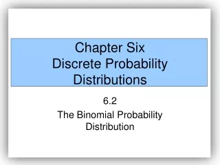
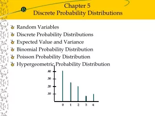
Binomial Experiments-I • Binomial experiments are those for which the outcome from each trial is one of only two options (“success” or “failure”). The properties of a binomial experiment are: • The experiment is repeated for a fixed number of trials, where each trial is independent of all the others. • There are only two possible outcomes for each trial. The outcomes can be classified as a success (S) or a failure (F). • The probability of success is the same for all trials. • The random variable X counts the number of successful trials out of n trials.
Binomial Experiments-II • Why is the following a binomial experiment? • We randomly sample 500 fish from the population. • We record whether each animal is mature or immature. • The random variable X is the number of mature animals.
Binomial Experiments-II(Notation) The experiment is repeated for a fixed number of trials There are only two possible outcomes (S and F) The probability of success P(S) is the same for each trial The random variable x counts the number of successful trials New terms
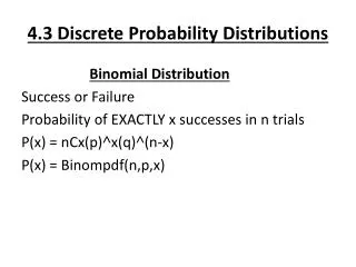
Binomial Probabilities-I • In a binomial experiment, the probability of exactly x successes in n trials is: • The binomial probability therefore involves the probability of x successes and n -x failures multiplied by the number of ways choosing x successes out of n trials. • n and p are known as parameters. Much of statistics involves using data to estimate the values for unknown parameters.
Binomial Probabilities-II • Notation: We read this as “The random variable X is distributed binomially with parameters n and p”.
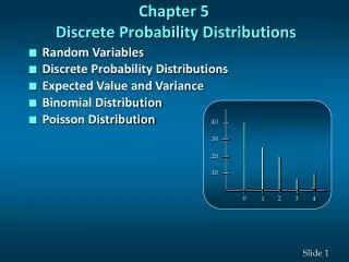
Binomial Probabilities-III • By listing all possible values of x with the corresponding probability of each, you can construct a . binomial probability distribution
Binomial Probabilities-IV • There is a probability of 0.2 that a fish in a given population has a particular disease. Assuming that 5 fish are sampled, construct the binomial probability distribution for the experiment. • What does this tell you about a sample size of 5 in this case?
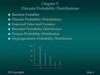
The Binomial Distribution n=6; p=0.5 n=6; p=0.7 0 1 2 3 4 5 6 0 1 2 3 4 5 6 n=6; p=0.9 0 1 2 3 4 5 6
Examples of the Binomial Distribution-I • We examine 12 animals for the presence of a disease (p=0.1). What is the probability that: • We find exactly 2 animals with the disease? • We find no animals with the disease? • We find 2 or more animals with the disease? • How many animals do we need to examine to be 99% sure that at least one has the disease?
Examples of the Binomial Distribution-II 0 1 2 3 4 5 6 7 8 9 10 11 12 Hint: I used the EXCEL function “COMBIN(N,x)”
Examples of the Binomial Distribution-III • P[X=2]= • P[X=0]= • P[X2]=1-P[X=0]-P[X=1]=0.3410 • We want to find n such that 1-P[X=0] < 0.01. This leads to n=40.
The Negative Binomial Distribution-I • We have an experiment with two outcomes: success (with probability p) and failure (with probability q =1-p). • Let r be a fixed number of successes, and the random variable X be the number of failures before we have r successes. • The probability distribution for X is:
The Negative Binomial Distribution-II • The product term is multiplied by and not because the final success is always the result of the last “trial” so we “know” when the last success occurs.
The Geometric Distribution-I • This is a special case of the negative binomial distribution for which r =1 (i.e. the probability of the number of failures until one success is recorded). • What then is the probability of finding the first diseased animal after finding five that are not diseased?
The Geometric Distribution-II • The Geometric distribution can be developed from the assumptions that: • A trial is repeated until a success occurs. • The repeated trials are independent of each other. • The probability of success p is constant for each trial.
The Geometric Distribution-III • What is the probability that the first diseased fish is not one of the first four examined? • This is equivalent to saying that the number of failures is NOT 0, 1, 2, or 3, i.e.: