Download
1 / 17
170 likes | 177 Vues
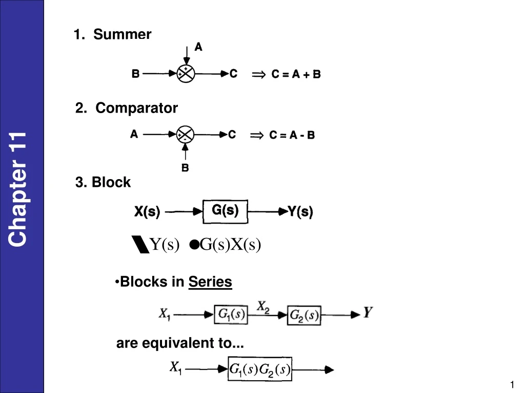
1. Summer. 2. Comparator. Chapter 11. 3. Block. Blocks in Series. are equivalent to. Figure 11.10 Three blocks in series. Figure 11.11 Equivalent block diagram. Block Diagram Reduction

E N D
1. Summer 2. Comparator Chapter 11 3. Block • Blocks in Series are equivalent to...
Figure 11.10 Three blocks in series. Figure 11.11 Equivalent block diagram.
Block Diagram Reduction In deriving closed-loop transfer functions, it is often convenient to combine several blocks into a single block. For example, consider the three blocks in series in Fig. 11.10. The block diagram indicates the following relations: By successive substitution, or where
Figure 11.8 Standard block diagram of a feedback control system.
Closed-Loop Transfer Functions The block diagrams considered so far have been specifically developed for the stirred-tank blending system. The more general block diagram in Fig. 11.8 contains the standard notation:
Set-Point Changes Next we derive the closed-loop transfer function for set-point changes. The closed-loop system behavior for set-point changes is also referred to as the servomechanism (servo) problem in the control literature. Combining gives
Figure 11.8 also indicates the following input/output relations for the individual blocks: Combining the above equations gives
Rearranging gives the desired closed-loop transfer function, Disturbance Changes Now consider the case of disturbance changes, which is also referred to as the regulator problem since the process is to be regulated at a constant set point. From Fig. 11.8, Substituting (11-18) through (11-22) gives
Because Ysp = 0 we can arrange (11-28) to give the closed-loop transfer function for disturbance changes: A comparison of Eqs. 11-26 and 11-29 indicates that both closed-loop transfer functions have the same denominator, 1 + GcGvGpGm. The denominator is often written as 1 + GOL where GOL is the open-loop transfer function, At different points in the above derivations, we assumed that D = 0 or Ysp = 0, that is, that one of the two inputs was constant. But suppose that D≠ 0 and Ysp ≠ 0, as would be the case if a disturbance occurs during a set-point change. To analyze this situation, we rearrange Eq. 11-28 and substitute the definition of GOL to obtain
Thus, the response to simultaneous disturbance variable and set-point changes is merely the sum of the individual responses, as can be seen by comparing Eqs. 11-26, 11-29, and 11-30. This result is a consequence of the Superposition Principle for linear systems.
“Closed-Loop” Transfer Functions • Indicate dynamic behavior of the controlled process • (i.e., process plus controller, transmitter, valve etc.) • Set-point Changes (“Servo Problem”) Assume Ysp 0 and D = 0 (set-point change while disturbance change is zero) Chapter 11 (11-26) • Disturbance Changes (“Regulator Problem”) Assume D 0 and Ysp = 0 (constant set-point) (11-29) *Note same denominator for Y/D, Y/Ysp.
General Expression for Feedback Control Systems Closed-loop transfer functions for more complicated block diagrams can be written in the general form: where:
Example 11.1 Find the closed-loop transfer function Y/Yspfor the complex control system in Figure 11.12. Notice that this block diagram has two feedback loops and two disturbance variables. This configuration arises when the cascade control scheme of Chapter 16 is employed. Figure 11.12 Complex control system.
Solution Using the general rule in (11-31), we first reduce the inner loop to a single block as shown in Fig. 11.13. To solve the servo problem, set D1 = D2 = 0. Because Fig. 11.13 contains a single feedback loop, use (11-31) to obtain Fig. 11.14a. The final block diagram is shown in Fig. 11.14b with Y/Ysp = Km1G5. Substitution for G4 and G5 gives the desired closed-loop transfer function: