Download
1 / 42
450 likes | 838 Vues
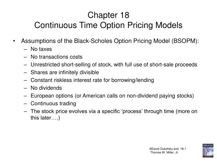
Chapter 18 Continuous Time Option Pricing Models. Assumptions of the Black-Scholes Option Pricing Model (BSOPM): No taxes No transactions costs Unrestricted short-selling of stock, with full use of short-sale proceeds Shares are infinitely divisible

E N D
Chapter 18Continuous Time Option Pricing Models • Assumptions of the Black-Scholes Option Pricing Model (BSOPM): • No taxes • No transactions costs • Unrestricted short-selling of stock, with full use of short-sale proceeds • Shares are infinitely divisible • Constant riskless interest rate for borrowing/lending • No dividends • European options (or American calls on non-dividend paying stocks) • Continuous trading • The stock price evolves via a specific ‘process’ through time (more on this later….)
Derivation of the BSOPM • Specify a ‘process’ that the stock price will follow (i.e., all possible “paths”) • Construct a riskless portfolio of: • Long Call • Short D Shares • (or, long D Shares and write one call, or long 1 share and write 1/D calls) • As delta changes (because time passes and/or S changes), one must maintain this risk-free portfolio over time • This is accomplished by purchasing or selling the appropriate number of shares.
The BSOPM Formula where N(di) = the cumulative standard normal distribution function, evaluated at di, and: N(-di) = 1-N(di)
The Standard Normal Curve • The standard normal curve is a member of the family of normal curves with μ = 0.0 and = 1.0. The X-axis on a standard normal curve is often relabeled and called ‘Z’ scores. • The area under the curve equals 1.0. • The cumulative probability measures the area to the left of a value of Z. E.g., N(0) = Prob(Z) < 0.0 = 0.50, because the normal distribution is symmetric.
The Standard Normal Curve The area between Z-scores of -1.00 and +1.00 is 0.68 or 68%. The area between Z-scores of -1.96 and +1.96 is 0.95 or 95%. Note also that the area to the left of Z = -1 equals the area to the right of Z = 1. This holds for any Z. What is N(1)? What is N(-1)? What is the area in each tail? What is N(1.96)? What is N(-1.96)?
Cumulative Normal Table(Pages 560-561) N(-d) = 1-N(d) N(-1.34) = 1-N(1.34)
Example Calculation of the BSOPM Value • S = $92 • K = $95 • T = 50 days (50/365 year = 0.137 year) • r = 7% (per annum) • s = 35% (per annum) What is the value of the call?
Solving for the Call Price, I. • Calculate the PV of the Strike Price: Ke-rT = 95e(-0.07)(50/365) = (95)(0.9905) = $94.093. • Calculate d1 and d2: d2 = d1–σT.5 = -0.1089 – (0.35)(0.137).5 = -0.2385
Solving for N(d1) and N(d2) • Choices: • Standard Normal Probability Tables (pp. 560-561) • Excel Function NORMSDIST • N(-0.1089) = 0.4566; N(-0.2385) = 0.4058. • There are several approximations; e.g. the one in fn 8 (pg. 549) is accurate to 0.01 if 0 < d < 2.20: N(d) ~ 0.5 + (d)(4.4-d)/10 N(0.1089) ~ 0.5 + (0.1089)(4.4-0.1089)/10 = 0.5467 Thus, N(-0.1089) ~ 0.4533
Solving for the Call Value C = S N(d1) – Ke-rT N(d2) = (92)(0.4566) – (94.0934)(0.4058) = $3.8307. Applying Put-Call Parity, the put price is: P = C – S + Ke-rT = 3.8307 – 92 + 94.0934 = $5.92.
Lognormal Distribution • The BSOPM assumes that the stock price follows a “Geometric Brownian Motion” (see http://www.stat.umn.edu/~charlie/Stoch/brown.htmlfor a depiction of Brownian Motion). • In turn, this implies that the distribution of thereturns of the stock, at any future date, will be “lognormally” distributed. • Lognormal returns are realistic for two reasons: • if returns are lognormally distributed, then the lowest possible return in any period is -100%. • lognormal returns distributions are "positively skewed," that is, skewed to the right. • Thus, a realistic depiction of a stock's returns distribution would have a minimum return of -100% and a maximum return well beyond 100%. This is particularly important if T is long.
BSOPM Properties and Questions • What happens to the Black-Scholes call price when the call gets deep-deep-deep in the money? • How about the corresponding put price in the case above? [Can you verify this using put-call parity?] • Suppose s gets very, very close to zero. What happens to the call price? What happens to the put price? Hint:Suppose the stock price will not change from time 0 to time T. How much are you willing to pay for an out of the money option? An in the money option?
Volatility • Volatility is the key to pricing options. • Believing that an option is undervalued is tantamount to believing that the volatility of the rate of return on the stock will be less than what the market believes. • The volatility is the standard deviation of the continuously compounded rate of return of the stock, per year.
Estimating Volatility from Historical Data 1.Take observations S0, S1, . . . , Sn at intervals of t (fractional years); e.g., t = 1/52 if we are dealing with weeks; t = 1/12 if we are dealing with months. 2. Define the continuously compounded return as: 3. Calculate the average rate of return 4. Calculate the standard deviation, s , of the ri’s 5. Annualize the computed s (see next slide). ; on an ex-div day:
Annualizing Volatility • Volatility is usually much greater when the market is open (i.e. the asset is trading) than when it is closed. • For this reason, when valuing options, time is usually measured in “trading days” not calendar days. • The “general convention” is to use 252 trading days per year. What is most important is to be consistent. Note that σyr > σmo > σweek > σday
Implied Volatility • The implied volatility of an option is the volatility for which the BSOPM value equals the market price. • The is a one-to-one correspondence between prices and implied volatilities. • Traders and brokers often quote implied volatilities rather than dollar prices. • Note that the volatility is assumed to be the same across strikes, but it often is not. In practice, there is a “volatility smile”, where implied volatility is often “u-shaped” when plotted as a function of the strike price.
Using Observed Call (or Put) Option Prices to Estimate Implied Volatility • Take the observed option price as given. • Plug C, S, K, r, T into the BSOPM (or other model). • Solving s (this is the tricky part) requires either an iterative technique, or using one of several approximations. • The Iterative Way: • Plug S, K, r, T, and into the BSOPM. • Calculate (theoretical value) • Compare (theoretical) to C (the actual call price). • If they are really close, stop. If not, change the value of and start over again.
Volatility Smiles In this table, the option premium column is the average bid-ask price for June 2000 S&P 500 Index call and put options at the close of trading on May 16, 2000. The May 16, 2000 closing S&P 500 Index level was 1466.04, a riskless interest rate of 5.75%, an estimated dividend yield of 1.5%, and T = 0.08493 year.
Graphing Implied Volatility versus Strike (S = 1466): Using the call data: α= 2.17;β1 = -4.47; β2 = 2.52; R2 = 0.988
Dividends • European options on dividend-paying stocks are valued by substituting the stock price less the present value of dividends into Black-Scholes. • Also use S* when computing d1 and d2. • Only dividends with ex-dividend dates during life of option should be included. • The “dividend” should be the expected reduction in the stock price expected. • For continuous dividends, use S* = Se-dT, where d is the annual constant dividend yield, and T is in years. Where: S* = S – PV(divs) between today and T.
The BOPM and the BSOPM, I. • Note the analogous structures of the BOPM and the BSOPM: C = SΔ + B (0< Δ<1; B < 0) C = SN(d1) – Ke-rTN(d2) • Δ = N(d1) • B = -Ke-rTN(d2)
The BOPM and the BSOPM, II. • The BOPM actually becomes the BSOPM as the number of periods approaches ∞, and the length of each period approaches 0. • In addition, there is a relationship between u and d, and σ, so that the stock will follow a Geometric Brownian Motion. If you carve T years into n periods, then:
The BOPM and the BSOPM: An Example • T = 7 months = 0.5833, and n = 7. • Let μ = 14% and σ = 0.40 • Then choosing the following u, d, and q will make the stock follow the “right” process for making the BOPM and BSOPM consistent:
Generalizing the BSOPM • It is important to understand that many option pricing models are related. • For example, you will see that many exotic options (see chap. 20) use parts of the BSOPM. • The BSOPM itself, however, can be generalized to encapsulate several important pricing models. • All that is needed is to change things a bit by adding a new term, denoted by b.
The Generalized Model Can Price European Options on: • Non-dividend paying stocks [Black and Scholes (1973)] • Options on stocks (or stock indices) that pay a continuous dividend [Merton (1973)] • Currency options [Garman and Kohlhagen (1983)] • Options on futures [Black (1976)]
By Altering the ‘b’ term in These Equations, Four Option-Pricing Models Emerge. By Setting:Yields this European Option Pricing Model:b = r Stock option model, i.e., the BSOPM b = r - d Stock option model with continuous dividend yield, d (see section 18.5.2) b = r – rf Currency option model where rf is the foreign risk-free rate b = 0 Futures option model
American Options • It is computationally difficult to value an American option (a call on a dividend paying stock, or any put). • Methods: • Pseudo-American Model (Sect. 18.10.1) • BOPM (Sects. 17.3.3, 17.4) • Numerical methods • Approximations • Of course, computer programs are most often used.
Some Extra Slides on this Material • Note: In some chapters, we try to include some extra slides in an effort to allow for a deeper (or different) treatment of the material in the chapter. • If you have created some slides that you would like to share with the community of educators that use our book, please send them to us!
The Stock Price Process, I. • The percent change in the stock prices does not depend on the price of the stock. • Over a small interval, the size of the change in the stock price is small (i.e., no ‘jumps’) • Over a single period, there are only TWO possible outcomes.
The Stock Price Process, II. • Consider a stock whose current price is S • In a short period of time of length Dt, the change in the stock price is assumed to be normal with mean of m S Dt and standard deviation, • m is expected return and s is volatility
That is, the Black-Scholes-Merton model assumes that the stock price, S, follows a Geometric Brownian motion through time:
Example: • Suppose Dt is one day. • A stock has an expected return of m = 0.0005 per day. • NB: (1.0005)365 – 1 = 0.20016, 20% • The standard deviation of the stock's daily return distribution is 0.0261725 • NB: This is a variance of 0.000685 • Annualized Variance: (365)(0.000685) = 0.250025 • Annualized STDEV: • (0.250025)0.5 = 0.500025, or 50% • (0.0261725)(365)0.5 = 0.500025, or 50%
Example, II. • Then, the return generating process is such that each day, the return consists of: • a non-stochastic component, 0.0005 or 0.05% • a random component consisting of: • The stock's daily standard deviation times the realization of Dz, • Dz is drawn from a normal probability distribution with a mean of zero and a variance of one. • Then, we can create the following table:
The First 10 Days of a Stochastic Process Creating Stock Returns: NON‑STOCHASTIC STOCHASTIC S(T)=S(T‑1)[1.0+R] TREND PRICE COMPONENT R = mDt + sDz DAY Dz S(T)=S(T‑1)[1.00050] (0.0261725)Dz Dt = 1 DAY 0 1.000000 1.000000 1 ‑2.48007 1.000500 ‑0.064910 0.935590 2 ‑0.87537 1.001000 ‑0.022911 0.914623 3 ‑0.80587 1.001501 ‑0.021092 0.895789 4 ‑1.03927 1.002002 ‑0.027200 0.871871 5 0.10523 1.002503 0.002754 0.874709 6 0.66993 1.003004 0.017534 0.890483 7 ‑0.21137 1.003505 ‑0.005532 0.886002 8 2.19733 1.004007 0.057510 0.937398 9 ‑0.82807 1.004509 ‑0.021673 0.917551 10 0.58783 1.005011 0.015385 0.932126
Risk-Neutral Valuation • The variable m does not appear in the Black-Scholes equation. • The equation is independent of all variables affected by risk preference. • The solution to the differential equation is therefore the same in a risk-free world as it is in the real world. • This leads to the principle of risk-neutral valuation. Applying Risk-Neutral Valuation: 1. Assume that the expected return from the stock price is the risk-free rate. 2. Calculate the expected payoff from the option. 3. Discount at the risk-free rate.
Two Simple and Accurate Approximations for Estimating Implied Volatility 1. Brenner-Subramanyam formula. Suppose:
Let’s Have a Horse Race • Data: S =54, K = 55, C = 1.4375, 29 days to expiration (T=29/365), r = 3%. We can verify: • The actual ISD is 30.06%. • Brenner-Subramanyam estimated ISD is 23.67%. • Corrado-Miller estimated ISD is 30.09%.