Download
1 / 85
850 likes | 1.07k Vues
Reloaded. Combinatorial Auctions. Review. Review. Optimal allocation Special case: Single minded bidders Incentive compatibility. Review. Greedy algorithm (single minded) LPR & DLPR Walrasian Equilibrium Every bidder receives his demand “demand” = maximum utility bundle

E N D
Reloaded Combinatorial Auctions
Review • Optimal allocation • Special case: Single minded bidders • Incentive compatibility
Review • Greedy algorithm (single minded) • LPR & DLPR • Walrasian Equilibrium • Every bidder receives his demand • “demand” = maximum utility bundle • Poly-time optimal allocation
Review Social welfare Linear program relaxation (LPR) Item cannot be more than once Bidder has at most one bundle Social welfare
Review Dual linear program relaxation (DLPR)
Lecture outline • “The curse of dimensionality” • Bidding languages • Iterative auctions • Queries • Communication complexity • Ascending auctions
The curse of dimensionality • High-dimensional input data • for all and • LPR • High dimensional solution vector • for all and • DLPR • Enormous amount of constraints Bidding languages Iterative auction
Goals • Expressiveness • What kind of valuations can we express? • Compactness • Use less bits for “interesting” kinds of valuations
OR bids • Any subset can be fulfilled • Example • ({a,b}, 12) OR ({c,d}, 8}) • Valuations • v({a}) = 0 • v({a,b}) = 12 • v({a,b,c}) = 12 • v({a,b,c,d}) = 12 + 8 = 20
OR bids • Formal definition • are called atomic bids. • Intuitively • Take all “valid” collections of items • Choose the one that has maximum value
XOR bids • Only one subset can be fulfilled • Choose maximum-value subset • Example • ({a,b}, 12)XOR({c,d}, 8) • Valuations • v({a,b}) = 12 • v{c,d}) = 8 • v({a,b,c,d}) = 12
Expression power • XOR bids can represent any valuation • Just XOR all possible values for all subsets • Can be very inefficient • OR bids – super additive valuations • implies
Expression power • Additive valuation • Naturally represented by OR bid • Unit-demand valuation • Naturally represented by XOR bid
OR/XOR combinations • Defined inductively • Let be valuations • Have more representation power
OR/XOR expression power • Symmetric valuation • depends only on • Downward sloping • Can be represented as with • Downward sloping with cannot be represented by OR bids and needs exponential size XOR bids.
OR/XOR expression power • Theorem • OR of XOR bids can express any downward-sloping symmetric valuation of items in size • Proof – next slide
OR/XOR expression power • For each define a clause that offers for any single item • Define the final expression as • Since are non-increasing – first item taken from the second from and so on
OR/XOR expression power • Example • We have 3 items and we have , and • The expression is
Dummy items • Goal – reuse single-minded allocation algorithm for OR/XOR bids • Method – represent everything as OR bids • Key observation • OR bids look like a collection of single-minded bids from different players.
Dummy items • How? Use dummy items! • Example • We have • Add a dummy item d • Rewrite as • Apply recursively for OR/XOR bids • We call this OR* bids
Dummy items • Theorem: Any valuation that can be represented by OR/XOR formula of size can be represented by OR* formula of size using at most dummy items • Remarks • A valuation in terms of the original formula is translated to in terms of OR* formula, where is the set of all dummy items. • The “size” of a formula is the amount of atomic bids it contains.
Dummy items • Two stage proof • (1) Prove that we can construct an OR* formula of size s • (2) Prove that we need at-most dummy items in the OR* formula.
Dummy items • Proof of (1) by induction • Definition • to be the OR* translation of v. • Base • A single pair is also an OR* bid • Step for • Let and • Define to be the union of atomic bids in and . • We got a formula of the same size as .
Dummy items • Example for XOR • Define dummy items • Translates to
Dummy items • Step for • Define and • Create dummy items for each pair of atomic bids in and in • Create • Transform each in to become • Similarly, transform each in • We got to be of the same size as.
Dummy items • Proof of (2) • Dummy item’s purpose is to disallow two atomic bids to be taken concurrently. • Thus we need dummy items – one for each pair of atomic bids that cannot be taken concurrently.
Dummy items • Conclusion: Every algorithm that can handle single-minded bids in polynomial time can handle any OR/XOR combinations in polynomial time.
Motivation • Reduce the amount of information transfer • Query mechanism that transmits less bits than OR/XOR? • Expressive power • Preserve some privacy • Bidder limitations • Bidders don’t know their valuation • Need effort to determine valuations • Guide bidders to the data relevant to the mechanism
Goals • Computational efficiency • How much information is transferred? • How long does it take to determine an allocation? • Incentive compatibility • Why should the bidders answer the queries truthfully?
Queries • The method of “asking for preferences” • Value query • What is the value of a bundle S? • Demand query • What would you like to buy for those prices? • Formally: Given a set of prices , what is the bundle S that maximizes
Expressive power • Demand queries are more powerful than value queries • Lemma: • A value query may be simulated using demand queries, where is the number of bits in the representation of bundle’s value. • Exponential number of value queries may be needed to simulate a single demand query. • Demand queries allow solving the LPR problem efficiently
Solve the linear program • Solve the DLPR • Use a method that doesn’t need all constraints at once • exponential amount of constraints! • Ellipsoid method to the rescue! • Use the solution of DLPR to solve LPR
Ellipsoid method • Solved LP problems by shrinking an ellipsoid • High level overview • Start with an ellipsoid that contains the solution. • Iteratively create a sequence such that: • contains the solution • results from constraint violation test
Solve the linear program • Ellipsoid method requirements • Given report weather is feasible or find a single constraint that violates. • DLPR constraints • Treat as utility and as prices • Constraint violation checking – using demand queries.
Solve the linear program • Demand-query all bidders using the prices . The results are . • Calculate • Using demand queries • Using a value query • If for all have a feasible point • Otherwise – we have a violated constraint.
Solving the primal • LP • Maximize • Subject to • Dual • Minimize • Subject to
Solving the primal c b A
Solving the primal c b A
Solving the primal c b A
Solving the primal • Use violated constraints from the Ellipsoid algorithm • Remove all other constraints still the same solution • Ellipsoid algorithm will produce the same final ellipsoid
Solving the primal c b A
Solving the primal c b A
Solving the primal • Solve the reduced-primal with polynomial number of variables! • Assign 0 to the unused ones.
Conclusions • Facts • WalrasianEquillibrium LPR has integer solution LPR solved optimal allocation • LPR can be solved in polynomial time • LPR solution requires polynomial number of demand queries. • Conclusion • WalrasianEquillibrium Can use demand queries to find optimal allocation in poly-time using polynomial amount of queries.