Download
1 / 26
260 likes | 432 Vues
Cht. IV The Equation of Motion. Prof. Alison Bridger 10/2011. Overview. In this chapter we will: Develop - using Newton’s 2nd Law of Motion - an equation that in principal - will enable us to predict flows.

E N D
Cht. IV The Equation of Motion Prof. Alison Bridger 10/2011
Overview • In this chapter we will: • Develop - using Newton’s 2nd Law of Motion - an equation that in principal - will enable us to predict flows. • Identify the forces which cause air motions. • Adapt the resulting equation to Earth. • See how the various forces work. • See what the resulting equation(s) look like in component form.
Introduction • In the previous chapter, a flow was assumed. • In this chapter we will develop an equation to predict the flow of air • This is called the Momentum Equation, or the Equation of Motion.
Introduction • In the next chapter, we’ll begin the process of solving this equation. • NOTE: flow evolution also depends on thermodynamic variables. • For example, we know (MET 61) that flows are forced by pressure gradients which follow from heating variations.
Introduction • In other chapter of CAR we will develop additional equations that forecast the entire evolution of the flow - dynamic and thermodynamic (via the variables V, p, T, etc.). • The entire set of equations are called the Equations of Motion.
Newton’s 2nd Law of Motion • Read the full definition on p. 142. • We have:
Newton’s 2nd Law of Motion • We sum over all possible forces (“Fi”) per unit mass. • If we can solve – integrate over time – we gain knowledge of the future velocity of the air parcel. • Speed & direction.
Newton’s 2nd Law of Motion • Here are some steps we need to follow: • identify the forces that affect air parcel motions • formulate how these work (mathematically) • substitute these forms back into the Eqn. above (“F=ma”), and then...
Newton’s 2nd Law of Motion • There is a problem (of course!) • Earth is rotating - this makes it a non-inertial frame of reference. • However, Newton’s 2nd Law is formulated for an inertial frame of reference.
Newton’s 2nd Law of Motion • Thus we must “adapt” the equation that we have developed to a non-inertial frame of reference. • This introduces the Coriolis force!
Forces... • We can start by identifying 2 basic types of forces: • body forces… • affect the entire body of the fluid (not just the surface) • act at a distance
Forces... • examples are • gravitational forces (not the same as gravity!) • magnetic forces • electrical forces • we ignore the latter two (lower atmosphere only!)
Forces... • surface forces… • affect the surface of a fluid parcel • caused by contact between fluid parcel • examples are • pressure forces • viscous forces (friction)
Gravitation • Newton’s Law of Gravitation…p.137 • the magnitude of the force is given by • Ga = GmM / r2 • G is the Universal Gravitation Constant • m and M are the two masses • r is the distance between the two centers of masses
Gravitation • We assume M = Earth’s mass (so MMe) and m = mass of air parcel (we will soon set m=1). • For the force direction, we assume: • Earth is a sphere • Earth is not rotating • Earth is homogeneous (so the center of mass is at the Earth’s geometric center) • As a result, we can write:
Gravitation • For the case m=1 (unit mass), Ga ga and we have:
Gravitation • Here, Ge is Earth’s Gravitation Constant (=GMe). • And note that the lower case (ga) means “per unit mass”. • So - the expression above for gagoes into the RHS of our expression of Newton’s 2nd Law (above).
Friction • This topic will be treated in detail in MET 130 etc. • In dynamics we typically take one of two approaches: • ignore friction - it’s usually a “second order” correction to the “important” “first-order” dynamics • assume something very simple for friction
Friction • example…we may set friction to depend linearly on the strength of the existing wind, as in
Friction • Here, is a constant that determines the rate of decay of V with time due to friction. • When we wish to allow for friction in our work, we will often simply add “F” to our Eqn. Of Motion - you should remember that “F” stands for friction.
Pressure Gradient Force • The last force important in driving motions is the pressure gradient force. • In many respects, it is the most important force since it initiates motions! • It is important to remember that it is pressure gradients that matter - not actual pressures themselves.
Pressure Gradient Force • Fluid parcels experience pressure forces due to contact with surrounding parcels. • When these forces are spatially variable, the parcel will experience a net motion. • We need to quantify this...