Lecture 22: Query Execution

1. Lecture 22:Query Execution Wednesday, November 19, 2003

2. Outline • Query execution: 15.1 – 15.5

3. Nested Loop Joins • Tuple-based nested loop R ⋈ S • Cost: T(R) B(S) when S is clustered • Cost: T(R) T(S) when S is unclustered for each tuple r in R do for each tuple s in S do if r and s join then output (r,s)

4. Nested Loop Joins • We can be much more clever • Question: how would you compute the join in the following cases ? What is the cost ? • B(R) = 1000, B(S) = 2, M = 4 • B(R) = 1000, B(S) = 3, M = 4 • B(R) = 1000, B(S) = 6, M = 4

5. Nested Loop Joins • Block-based Nested Loop Join for each (M-2) blocks bs of S do for each block br of R do for each tuple s in bs for each tuple r in br do if r and s join then output(r,s)

6. . . . Nested Loop Joins Join Result R & S Hash table for block of S (M-2 pages) . . . . . . Output buffer Input buffer for R

7. Nested Loop Joins • Block-based Nested Loop Join • Cost: • Read S once: cost B(S) • Outer loop runs B(S)/(M-2) times, and each time need to read R: costs B(S)B(R)/(M-2) • Total cost: B(S) + B(S)B(R)/(M-2) • Notice: it is better to iterate over the smaller relation first • R ⋈ S: R=outer relation, S=inner relation

8. Two-Pass Algorithms Based on Sorting • Recall: multi-way merge sort needs only two passes ! • Assumption: B(R)<= M2 • Cost for sorting: 3B(R)

9. Two-Pass Algorithms Based on Sorting Duplicate elimination d(R) • Trivial idea: sort first, then eliminate duplicates • Step 1: sort chunks of size M, write • cost 2B(R) • Step 2: merge M-1 runs, but include each tuple only once • cost B(R) • Total cost: 3B(R), Assumption: B(R)<= M2

10. Two-Pass Algorithms Based on Sorting Grouping: ga, sum(b) (R) • Same as before: sort, then compute the sum(b) for each group of a’s • Total cost: 3B(R) • Assumption: B(R)<= M2

11. Two-Pass Algorithms Based on Sorting x = first(R) y = first(S) While (_______________) do{ case x < y: output(x) x = next(R) case x=y: case x > y;} R ∪ S Completethe programin class:

12. Two-Pass Algorithms Based on Sorting x = first(R) y = first(S) While (_______________) do{ case x < y: case x=y: case x > y;} R ∩ S Completethe programin class:

13. Two-Pass Algorithms Based on Sorting x = first(R) y = first(S) While (_______________) do{ case x < y: case x=y: case x > y;} R - S Completethe programin class:

14. Two-Pass Algorithms Based on Sorting Binary operations: R ∪ S, R ∩ S, R – S • Idea: sort R, sort S, then do the right thing • A closer look: • Step 1: split R into runs of size M, then split S into runs of size M. Cost: 2B(R) + 2B(S) • Step 2: merge M/2 runs from R; merge M/2 runs from S; ouput a tuple on a case by cases basis • Total cost: 3B(R)+3B(S) • Assumption: B(R)+B(S)<= M2

15. Two-Pass Algorithms Based on Sorting R(A,C) sorted on AS(B,D) sorted on B x = first(R) y = first(S) While (_______________) do{ case x.A < y.B: case x.A=y.B: case x.A > y.B;} R ⋈R.A =S.B S Completethe programin class:

16. Two-Pass Algorithms Based on Sorting Join R ⋈ S • Start by sorting both R and S on the join attribute: • Cost: 4B(R)+4B(S) (because need to write to disk) • Read both relations in sorted order, match tuples • Cost: B(R)+B(S) • Difficulty: many tuples in R may match many in S • If at least one set of tuples fits in M, we are OK • Otherwise need nested loop, higher cost • Total cost: 5B(R)+5B(S) • Assumption: B(R)<= M2, B(S)<= M2

17. Two-Pass Algorithms Based on Sorting Join R ⋈ S • If the number of tuples in R matching those in S is small (or vice versa) we can compute the join during the merge phase • Total cost: 3B(R)+3B(S) • Assumption: B(R)+ B(S)<= M2

18. Relation R Partitions OUTPUT 1 1 2 INPUT 2 hash function h . . . M-1 M-1 M main memory buffers Disk Disk Two Pass Algorithms Based on Hashing • Idea: partition a relation R into buckets, on disk • Each bucket has size approx. B(R)/M • Does each bucket fit in main memory ? • Yes if B(R)/M <= M, i.e. B(R) <= M2 1 2 B(R)

19. Hash Based Algorithms for d • Recall: d(R) = duplicate elimination • Step 1. Partition R into buckets • Step 2. Apply d to each bucket (may read in main memory) • Cost: 3B(R) • Assumption:B(R) <= M2

20. Hash Based Algorithms for g • Recall: g(R) = grouping and aggregation • Step 1. Partition R into buckets • Step 2. Apply g to each bucket (may read in main memory) • Cost: 3B(R) • Assumption:B(R) <= M2

21. Partitioned Hash Join R ⋈ S • Step 1: • Hash S into M buckets • send all buckets to disk • Step 2 • Hash R into M buckets • Send all buckets to disk • Step 3 • Join every pair of buckets

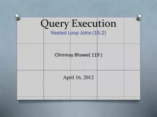
22. Original Relation Partitions OUTPUT 1 1 2 INPUT 2 hash function h . . . M-1 M-1 B main memory buffers Disk Disk Partitions of R & S Join Result Hash table for partition Si ( < M-1 pages) hash fn h2 h2 Output buffer Input buffer for Ri B main memory buffers Disk Disk Hash-Join • Partition both relations using hash fn h: R tuples in partition i will only match S tuples in partition i. • Read in a partition of R, hash it using h2 (<> h!). Scan matching partition of S, search for matches.

23. Partitioned Hash Join • Cost: 3B(R) + 3B(S) • Assumption: min(B(R), B(S)) <= M2

24. Hybrid Hash Join Algorithm • Partition S into k buckets • But keep first bucket S1 in memory, k-1 buckets to disk • Partition R into k buckets • First bucket R1 is joined immediately with S1 • Other k-1 buckets go to disk • Finally, join k-1 pairs of buckets: • (R2,S2), (R3,S3), …, (Rk,Sk)

25. Hybrid Join Algorithm • How big should we choose k ? • Average bucket size for S is B(S)/k • Need to fit B(S)/k + (k-1) blocks in memory • B(S)/k + (k-1) <= M • k slightly smaller than B(S)/M

26. Hybrid Join Algorithm • How many I/Os ? • Recall: cost of partitioned hash join: • 3B(R) + 3B(S) • Now we save 2 disk operations for one bucket • Recall there are k buckets • Hence we save 2/k(B(R) + B(S)) • Cost: (3-2/k)(B(R) + B(S)) = (3-2M/B(S))(B(R) + B(S))

27. Hybrid Join Algorithm • Question in class: what is the real advantage of the hybrid algorithm ?

28. a a a a a a a a a a Indexed Based Algorithms • Recall that in a clustered index all tuples with the same value of the key are clustered on as few blocks as possible • Note: book uses another term: “clustering index”. Difference is minor…

29. Index Based Selection • Selection on equality: sa=v(R) • Clustered index on a: cost B(R)/V(R,a) • Unclustered index on a: cost T(R)/V(R,a)

30. Index Based Selection • Example: B(R) = 2000, T(R) = 100,000, V(R, a) = 20, compute the cost of sa=v(R) • Cost of table scan: • If R is clustered: B(R) = 2000 I/Os • If R is unclustered: T(R) = 100,000 I/Os • Cost of index based selection: • If index is clustered: B(R)/V(R,a) = 100 • If index is unclustered: T(R)/V(R,a) = 5000 • Notice: when V(R,a) is small, then unclustered index is useless

31. Index Based Join • R ⋈ S • Assume S has an index on the join attribute • Iterate over R, for each tuple fetch corresponding tuple(s) from S • Assume R is clustered. Cost: • If index is clustered: B(R) + T(R)B(S)/V(S,a) • If index is unclustered: B(R) + T(R)T(S)/V(S,a)

32. Index Based Join • Assume both R and S have a sorted index (B+ tree) on the join attribute • Then perform a merge join (called zig-zag join) • Cost: B(R) + B(S)

33. Questions in Class • B(Product), B(Company) are large • Which join method would you use ? • Consider: • 10 bozosv.s. 100…0 • 10 coolcompaniesv.s. 100…00 SELECT Product.name, Company.cityFROM Product, CompanyWHERE Product.maker = Company.name and Product.category = ‘bozo’ and Company.rating = ‘cool’