Download
1 / 17
170 likes | 273 Vues
Warm-up Day before of Ch. 3 Test. The following data represent scores of 50 students on a Statistics Exam. 72 72 93 70 59 78 74 65 73 80 57 67 72 57 83 76 74 56 68 67 74 76 79 72 61 72 73 76 67 49 71 53 67 65 100 83 69 61 72 68 65 51 75 68 75 66 77 61 64 74.

E N D
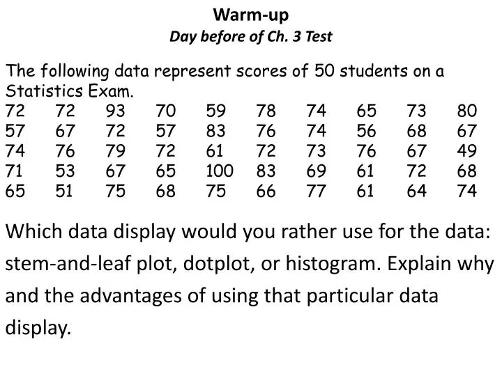
Warm-upDay before of Ch. 3 Test The following data represent scores of 50 students on a Statistics Exam. 72 72 93 70 59 78 74 65 73 80 57 67 72 57 83 76 74 56 68 67 74 76 79 72 61 72 73 76 67 49 71 53 67 65 100 83 69 61 72 68 65 51 75 68 75 66 77 61 64 74 Which data display would you rather use for the data: stem-and-leaf plot, dotplot, or histogram. Explain why and the advantages of using that particular data display.
A.P. Statistics Answer to #23 and #24 of Practice Test 24. a. The coefficient of correlation would be 0.997. This means that there is an extremely strong correlation between age and height in John’s childhood growth. b. The coefficient of determination is 99.6%. 99.6% of John’s height can be predicted from his age.
Statistics 3.4 Residual plot for #45 C. The skin sample with the unusually effective disinfectant would be the (8, 0). The skin sample with the least effective disinfectant would be the (10, 13). The coded bacteria colony increased after treatment!
Stats Answers to Practice Test 1) Time studying 9)B 2) mileage 10)C 3) volume 11)B 4) A and C 12)C 5)All false. B appears true BUT 6)A 7)C (since the * is on what would be the regression line, removing it would decrease correlation.) 8)C
A.P. Statistics P#26 pg 195 Dying dice. Imagine if someone with 200 die, when they are rolled only “1-4” live. Rolls with a 5 or 6 are removed. The number of live dice are recorded after each roll. Here are the results: 200, 122, 81, 58, 29, 19, 11, 8 ,6, 4, 2, 2 • Construct a scatterplot of the live dice. • Transform the scatter plot using ln. • Sketch the new scatterplot; write and sketch the linear regression line. • Use the calculator to graph the residual plot. Sketch your results and describe what you see.
A.P. Statistics 3.5 P #26 pg 194 Live Die 200, 122, 81, 58, 29, 19, 11, 8 ,6, 4, 2, 2 Roll 0, 1, 2, 3, 4, 5, 6, 7, 8, 9 10, 11 Sketch the residual plot and describe what you see.
A.P. Statistics H.W. • Complete #27 all parts - we will review the answers in 15 minutes • I will be calling the remaining people to see their notes. • When you are finished complete AP #1-8 on pg 212 -213
A.P. Statistics 3.5 P #27 • First you had to graph the data, to see if it looked exponential or like a power relationships. You should have determined it was an exponential growth function. Since it was exponential you should have used log or ln on the Y values to linearize the graph. • The equation of the linearized data would be ln(pop) = -54.9342 + 0.03583 year. The growth rate is 3.6%/year. c) The residual plot shows a pattern. On the residual plot you could see a big jump in growth occurred between 1950 and 1960. In 200 there was a big drop in growth.
Statistics Finish Practice Test #13 - 23 • Work on the 13 -23 quietly by yourself first for the first 30 minutes. • Then you will be allowed to discuss the problems at your table before seeing the answers • Have your notes ready.
Statistics Ch. 3 Quiz 1 # 3 - Revisited A student wonders if people of similar heights tend to date each other. She measures herself, her dormitory roommate, and the women in the adjoining rooms; then she measures the next man whom each woman dates. Here are the data (heights in inches): Women 64 65 65 66 66 70 Men 68 68 69 70 72 74 a. Plot the points so that the female height predicts her male date’s height. b. Compute the equation of the least squares regression line, and draw the line on your plot. c. Interpret the slope and y-intercept in the context of this situation. d. Using your line from part b, estimate the height of the male dating a 72 inch female. e. Calculate the residual for the 74 inch male. f. Verify that the least squares regression line goes through the point of averages, (x, y) . g. Verify that the sum of the residuals is 0.
Remaining Answers for Statistics 13)A & B can’t tell; C yes; D no-moderate 14)D 15) Driving experience 16) x-axis driving experience; y-axis premium $ Linear regression (0, 72.7) and (25, 40.2) 17) increase, decrease 18) -0.775 19) $59.70 20)Yes. The regression line is appropriate because the residual points are scattered are both sides radomly. 21)C 22) A
Statistics Answer to #23 and #24 of Practice Test 24. a. The coefficient of correlation would be 0.997. This means that there is an extremely strong correlation between age and height in John’s childhood growth. b. The coefficient of determination is 99.6%. 99.6% of John’s height can be predicted from his age.
Statistics Candy Grab Activity Redo • 4 students need to make-up the candy grab activity. • A couple of groups won’t be happy with their grade. These groups are welcome to stay during 7th block and redo the problems they got marked to earn ½ points back. Example: If your group got 15/25, they can get 5pts of the 10 back if all redone problems are correct. Their new score will be a 20/25 = 80%