Download
1 / 30
340 likes | 765 Vues
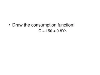
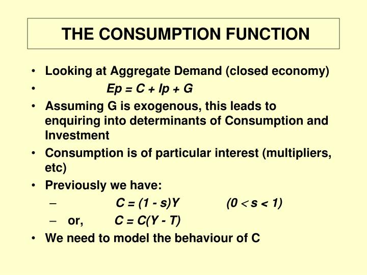
THE CONSUMPTION FUNCTION. Looking at Aggregate Demand (closed economy) Ep = C + Ip + G Assuming G is exogenous, this leads to enquiring into determinants of Consumption and Investment Consumption is of particular interest (multipliers, etc) Previously we have:

E N D
THE CONSUMPTION FUNCTION • Looking at Aggregate Demand (closed economy) • Ep = C + Ip + G • Assuming G is exogenous, this leads to enquiring into determinants of Consumption and Investment • Consumption is of particular interest (multipliers, etc) • Previously we have: • C = (1 - s)Y (0 s < 1) • or, C = C(Y - T) • We need to model the behaviour of C
EARLY FORMULATION: KEYNES (1936) • Keynes (1936) made three main assertions: • C = C(Y), (not r) • 0 MPC 1, (where MPC is dC/dY) • APC falls as Y increases (APC is C/Y) • Taken together these imply a Consumption Function of the form: C = A + bY • where A and b are positive constants • APC = A/Y + b • MPC = b • and A/Y must fall as Y increases
GRAPH OF THE BASIC CONSUMPTION FUNCTION • As Y increases, C/Y falls: also dC/dY C/Y C 45O C = A + bY dC/dY = b A 0 Y
EARLY EMPIRICAL EVIDENCE • Keynes hadn’t have much statistical evidence on consumption • Early estimates in the 1940s for the USA and elsewhere were conflicting. • Short-medium term annual data (1929-45) • C = A + bY; A 0; b 0.7 • Long-term data (1869-1945) • C = bY: A 0, b 0.9 • Which is “right”? • We need a proper model to answer this.
LONG AND MEDUIM RUN EVIDENCE ON CONSUMPTION • 1929-45: C = A + bY • 1869-45; C = b*Y C 45O b* 0.9 C = b* Y C = A + bY b 0.7 0 Y
MODELS OF AGGREGATE CONSUMPTION • Basic Intertemporal Choice model (Fisher) • The Life-Cycle theory of Consumption (Modigliani, etc) • The Permanent Income theory of Consumption (Friedman)
INTERTEMPORAL CHOICE • Generally we require: PV(C) or PV(Y) • i.e. C1 + C2 (1+r) or Y1 + Y2 (1+r) • or Ci (1+r)i or Yi (1+r)i • Households maximize Utility over expected lifetime • i.e. Max: U = U (C1, ..., Ci , ... , Cn) • s.t. Ci (1+r)i or Yi (1+r)i(i : 1 n)
INTERTEMPORAL CHOICE Indifference Curves represent U = U(C1 , C2 ) C2 C1 0
INTERTEMPORAL CHOICE Endowment at E: OB = PV(Y) = y1 + y2 (1 + r) Slope of AB is (1 + r) Y2 A . E y2 y1 Y1 0 B
INTERTEMPORAL CHOICE Why is slope AB = - (1 + r) ? Suppose (present) savings increase by €100 i.e. C1 = - 100 This allows an increase in C2 of 100(1 + r) i.e. C2 = +100 (1 + r) Slope AB = C2 C1 = 100 (1 + r)/ - 100 = - (1 + r)
A CHANGE IN r An increase in r: AB pivots at E CD Y2 C A . E y2 y1 Y1 0 D B
OPTIMAL C Saving is (oy1- oc*1) : future dis-saving is (oc*2 - oy2) Y2 A c*2 c* . y2 E 0 c*1 y1 B Y1
CHANGES IN Y AND C Y2 increases: E’ E”, AB CD, c’1 c”1 Y2 C A . E” . E’ 0 c’1 c”1 B D Y1
A INCREASE IN r : SAVER Income effect 1 3; Substitution effect 3 2 Y2 C F A 2 3 1 . y2 E 0 y1 Y1 c31 c21 D B G c11
A INCREASE IN r : BORROWER Inc. effect 1 2; Sub. effect 2 3 Y2 C A . F E 3 1 2 0 Y1 y1 c31 c11 c21 D G B
IMPERFECT CAPITAL MARKETS Borrowing rate (EB) > lending rate (AE) C2 A . Y2 E 0 Y1 B C1
CREDIT (BORROWING) CONSTRAINT . C2 I” Constraint: ADB I’ A Consumer cannot borrow more than Y1B E Y2 D 0 Y1 B C1
THE LIFE-CYCLE HYPOTHESIS • Income shows a marked life-cycle variation • It is low in the early years, reaches a peak in late middle age and declines, especially on retirement • Smoothing consumption over a lifetime is a rational strategy (diminishing MUy) • This implies C/Y will vary during the lifetime of an individual
THE LIFE-CYCLE HYPOTHESIS . C2 E’: low Y1/Y2 high C1/Y1 E”: high Y1/Y2 low C1/Y1 A E’ . C2* . E” C1 B 0 Y1’ C1* Y1”
THE LIFE-CYCLE HYPOTHESIS Y, C and W over the life-cycle Y, C Ct Yt Age 18 65 +W Wt Age W
THE LIFE-CYCLE MODEL • Let retirement age = 65; life expectancy = 75 • Years to retirement = R (= 65 – present age) • Expected life = T (= 75 – present age) • Assuming no pension, no discounting: • CT = W + RY is the lifetime constraint • i.e. C = (W + RY)/T • and C = (1/T)W + (R/T)Y • or C = W + Y ( = 1/T; = R/T)
THE LIFE-CYCLE MODEL • C = W + Y • MPC = C Y = • APC = C Y = (W Y) + • clearly MPC < APC • for a “typical” individual, age 35 • R=30, T = 40 • = 1/T 0.03; (MPC) = RT 0.75 • APC = [0.03 (W Y) + 0.75] > MPC
THE LIFE-CYCLE MODEL • Saving and Consumption behaviour may depend on population age-structure • Does Social Security displace personal savings? • What is the effect of Medicare (USA) or Medical Cards for over 70s (IRL) on Savings? • Savings and Uncertainty: • “rational” behaviour: run down wealth to zero • individual circumstances unpredictable (care needs) • individual life expectancy unpredictable • on average even selfish people will die with W > 0
THE PERMANENT INCOME HYPOTHESIS • Cp = kYp (0 k 1 ) • Y = Yp+ Ytr • C = Cp + Ctr • Permanent income is the return to all wealth, human and non-human: • Yp = rW • which implies: Cp = rkW • NB: C is not related to Ytr i.e. dC dYtr = 0
MEASURING PERMANENT INCOME AND CONSUMPTION (1) • Are Cpand Yp observable? • E(Ytr ) = 0 • E(Ctr ) = 0 • which imply that E(Y) = E(Yp ), etc. • However this is ex ante: ex post, actual measures may reveal more • (a) in a recession: Y < Yp : Ytr < 0 • (b) in a boom: Y > Yp : Ytr > 0
MEASURING PERMANENT INCOME AND CONSUMPTION (2) • Cross-section measurements of C and Y C 45o Ci, Yi. . . . . Ci = A + bYi . . Cm . 0 Y Ym
MEASURING PERMANENT INCOME AND CONSUMPTION (3) • Where Yj > Ym, Ytr > 0 and Yj > Ypj C 45o Cp =kYp Cj Ci = A + bYi Cm Ytrj 0 Y Yj Ym Ypj
MEASURING PERMANENT INCOME AND CONSUMPTION (4) • Aggregate: Ytr > 0 in boom, < 0 in recession • Measured C/Y should be < in boom than in recession (Recent experience?) • Aggregate Ctr = 0: individual Ctr is > or < 0 • Average Ctr = 0 for all income groups • Measuring Yp: • Adaptive expectations: Yp = f(Yt, Y t - 1, ...Y t-n) • Rational expectations: only new information (shocks) change Yp • Consumption V Consumption Expenditure, which highlights the role of durables (Investment and saving rather than consumption
MEASURING PERMANENT INCOME AND CONSUMPTION (5) • Also we may express the PYH as an error-correction model: • Ypt = Ypt-1 + j(Yt – Ypt-1) 0 < j < 1 • which with: Ct = Cpt = kYpt • gives: Ct = kYpt = kYpt-1 + kj(Yt – Ypt-1) • Re-arranging: Ct = (k – kj)Ypt-1 + kjYt • j 0 implies slow adaptation, j 1 implies rapid adaptation • assume k = 0.9, j = 0.3, so kj = 0.27 • then: Ct = (0.9 – 0.27)Ypt-1 + 0.27Yt or 0.63Ypt-1 + 0.27Yt • However this is not an explicitly forward-looking model. • Now suppose C = Cp = kYp, then Yp = 1/k(Cp) • Thus Ct = (0.63/k)Ct – 1 + 0.27Yt = 0.7Ct – 1 + 0.27Yt
PERMANENT INCOME AND RECESSION • Y < Yp in short-run (mild) recession • Suppose there is a shock to the system (financial crisis) • Pwople expect a severe long-drawn-out recession: i.e. Yp falls, ie. E(Y) falls • It is possible that initiallyY > Yp • C (and Cp) will fall • If people anticipate a fall in Yp, then C/Y may fall • Current (mid-2009) situation: big fall in W, both the Permanent and Life-cycle theories predict that this will hit C (independently of current measured Y)