Download
1 / 23
260 likes | 583 Vues
Convolution Shadow Maps. * MPI Informatik Germany. † Hasselt University Belgium. ‡ University College London UK. Motivation: Screen-space anti-aliasing. Percentage Closer Filtering (NVIDIA). Convolution Shadow Map (CSM). Shadow Mapping. Problem statement.

E N D
Convolution Shadow Maps *MPI Informatik Germany † Hasselt University Belgium ‡University College London UK
Motivation: Screen-space anti-aliasing Percentage Closer Filtering (NVIDIA) Convolution Shadow Map (CSM)
Shadow Mapping Problem statement Filtering the z values of the Shadow Map Filtering the CSM data structure Helix scene ? ?
Benefits of a CSM • Efficient screen-space anti-aliasing through hardware filtering • Including mipmapping and anisotropic filtering • Enables additional convolutions • Blur filter conceals discretization artifacts • Improves temporal coherence substantially
Related Work • Percentage Closer Filtering (PCF) [Reeves et al. 1987] • average multiple shadow tests • NVIDIA’s GPU version • 2x2 pattern • analogous to bilinear filter • Trilinear (mipmap) not possible • Variance Shadow Maps (VSM) [Donnelly et al. 2006] • Probabilistic approach • Filtering z and z2 • Estimates upper bound only • Light leaking artifacts • Precision problems Courtesy of Donnelly [Demo]
L p z(p) c d(x) x Shadow Mapping [Williams 1978] • xR3 • pR2 • x equals p just in different spaces • Shadow function:s(x):=f(d(x),z(p)) • Binary result: • 1 if d(x)<=z(p) • 0 else
L p d(x’) z(p) c x x’ Shadow test function: s(x) • What kind of function is s(x)? • Heaviside Step Function: H(t) Shadow term for x’
L p q p z(p) N c d(x) x y y N How to filter s(x) ? • Filter s(x) “around” p • Assume d(y)≈ d(x) • d(x) representativedistance forN • Same for PCF • Then we get:
f(d,z) = ai(d) Bi(z) s(x)≈ ai(d(x)) Bi(z(p)) Non-linearity of the shadow test • = • Filtering shadow test result != filtering z values • Our new solution: Transform depth map such that we can write the shadow test as a sum (1D function) z(p) Bi(z(p))
Reconstruction Example • s(x) ≈ a1(d) +a2(d) +..+ a4(d) +..+ a8(d) +..+a16(d)
= [w * ai(d(x)) Bi(z)](p) = ai(d(x))[w * Bi(z)](p) Why is this useful? • Fill expansion into convolution formula • Convolution on s(x) == convolution on Bi(z(p)) • Note: d(x) and z(p) had to be separable! • Decoupling d(x) and z(p) enables pre-filtering! sf (x) = [w * f(d(x), z)](p)
s(x) ≈ a1(d) +..+a4(d) +…+ a8(d) +..+a16(d) sf (x) ≈ a1(d) +..+a4(d) +…+ a8(d) +..+a16(d) Filtering Example Original Bi(z) After filtering Bi(z) [w * Bi(z)]
What expansion do we use? • Approximate shadow test with Fourier series c1 +c2 +..+c4 +..+c8 +..+c16
c1 +c2 +..+c4 +..+c8 +..+c16 Important properties of a Fourier series • Step function becomes sum of weighted sin() • Series is separable! • Constant error due to shift invariance
PCF (NVIDIA) Anti-aliased shadows (SM: 5122) • Trilinear filtering and additional convolution CSM CSM – 7x7 Gauss
PCF (NVIDIA) CSM CSM – 7x7 Gauss Tree scene (SM: 20482) • Mipmapped CSM recovers fine details
Blurred Shadows Filter size: 3x3 1282 2562 5122 10242 SM: Filter size:7x7 1282 2562 5122 10242 SM:
Issues with a Fourier series • Ringing suppression • Reduce higher frequencies • Steepness of “ramp” • Offset (transl. invariance!) • Shift shadow test • Increases lightness prob. • Scaling • Scale shadow test • Decreases filtering • See paper for tradeoffs
Limitations and drawbacks • Influence of reconstruction order M • Memory consumption increases as M grows • Performance (filtering) decreases as M grows M = 1 M = 2 M = 4 M = 8 M = 16
Performance and Memory • Frame rate for complex scene (see video) ~365k polygons (NVIDIA GeForce 8800-GTX) • Requires (M/2) 8-bit RGBA textures • Apply convolution to each texture 256 512 1024 2048
Conclusion • CSM, a new data structure which enables pre-filtering of shadow maps • Mipmaps • High quality screen-space anti-aliasing for shadow rendering • Improved temporal coherence • Additional convolution conceals discretization artifacts
Outlook and Extensions • New separable expansion • Less memory • Higher performance • Better quality at contact points • Rendering approximate Soft shadows • Efficient algorithm based on spatial relations